










SRTF Scheduling Examples
SRTF (Shortest Remaining Time First) Scheduling In OS is also known as Shortest Job First (SJF) with preemption. In the SRTF algorithm, any process that has the shortest remaining burst time is always executed first.
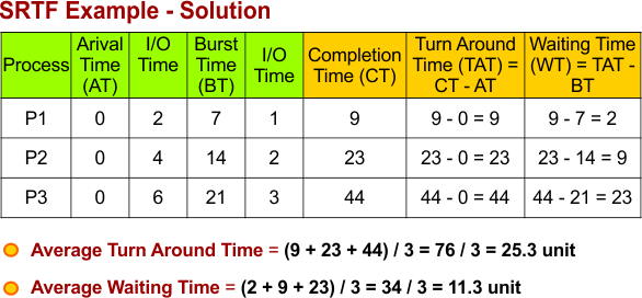
We will solve the examples of SRTF by using the following formulas, where the given information includes Process ID, Arrival Time, Burst Time, and optional I/O time
- Gets CPU First Time: It can be seen in the Gantt Chart directly, without using any formula
- Completion Time (CT): It can also be seen in the Gantt Chart directly, without using any formula
- Turnaround Time (TAT) = Completion Time (CT) − Arrival Time (AT)
- Waiting Time (WT) = Turnaround Time (TAT) − Burst Time (BT)
- Average Waiting Time (AWT) = Sum of all Waiting Times / Number of Processes
- Average Turnaround Time (ATAT) = Sum of all Turnaround Times / Number of Processes
- Response Time (RT) = First CPU Start Time − Arrival Time (AT)
Let’s explain some Examples of SRTF algorithm.
SRTF Scheduling Example 1
Consider the following table, which includes the Process, Arrival time, and burst time.
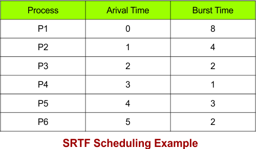
Gannt. Chart of the given example 1 is given below

The following diagram shows how to calculate the Completion Time (CT), Waiting Time (WT), Turnaround Time (TAT), Average Waiting Time (AWT), Average Turnaround Time (ATAT), and Response Time (RT).
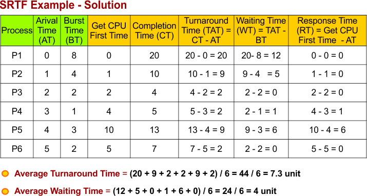
Explaination
At time 0
Only a single process P1 arrives in the ready queue at time 0; no other process arrives yet. CPU will start execution with P1
- Ready Queue: P1
At time 1
P2 arrives, containing a burst time of 4 units of time, which is less than P1 (contains burst time = 7, after executing 1 unit of time in the 0 to 1 period of time). So, the CPU switches to P2
- Ready Queue: P1, P2
At time 1, look at the Burst time of all processes
| Processes | Remaining Burst time |
| P1 | 7 |
| P2 | 4 |
At time 2
P3 arrives, which containing Burst time of 2 units of time, which is the shortest burst time among others. So, the CPU switches to P3
- Ready Queue: P1, P2, P3
At time 2, look at the Burst time of all processes
| Processes | Remaining Burst time |
| P1 | 7 |
| P2 | 3 |
| P3 | 2 |
At time 3
P4 arrives, which contains a burst time of 1 unit of time, which is not the shortest burst time among others.
- But P4 ties with P3 at time 3, because P3 and P4 both contain a similar burst time = 1 unit of time. We use any method (when not given in the question), i.e., the smaller process ID option to break the tie
So, the CPU continues with P3
- Ready Queue: P1, P2, P3, P4
At time 3, look at the Burst time of all processes
| Processes | Remaining Burst time |
| P1 | 7 |
| P2 | 3 |
| P3 | 1 |
| P4 | 1 |
At time 4
P3 completes its execution, and P5 arrives, which contains a burst time of 3 units of time, which is not the shortest burst time among others. So, the CPU switches to P4, which contains shortest burst time.
- Ready Queue: P1, P2, P4, P5
At time 4, look at the Burst time of all processes
| Processes | Remaining Burst time |
| P1 | 7 |
| P2 | 3 |
| P3 | Nil, Process Terminated |
| P4 | 1 |
| P5 | 3 |
At time 5
P4 completes its execution, and P6 arrives, which contains a burst time of 2 units of time, which is the shortest burst time among others.
So, the CPU switches to P6, which contains the shortest burst time.
- Ready Queue: P1, P2, P5, P6
At time 5, look at the Burst time of all processes
| Processes | Remaining Burst time |
| P1 | 7 |
| P2 | 3 |
| P3 | Nil, Process Terminated |
| P4 | Nil, Process Terminated |
| P5 | 3 |
| P6 | 2 |
At time 5 to 7:
P6 completes its execution at 7; no new process arrives. The ready queue contains only P1, P2, P5; where P2 and P5 tie in terms of burst time. We break the tie using arrival time. As P2 comes first, the CPU switches to P2 next
- Ready Queue: P1, P2, P5
At time 7, look at the Burst time of all processes
| Processes | Remaining Burst time |
| P1 | 7 |
| P2 | 3 |
| P3 | Nil, Process Terminated |
| P4 | Nil, Process Terminated |
| P5 | 3 |
| P6 | Nil, Process Terminated |
At time 7 to 10:
P2 completes its execution at 10; no new process arrives in time 7 to 10. The ready queue contains only P1 and P5; where P5 has the shortest remaining burst time, so it will be executed next
- Ready Queue: P1, P5
At time 10, look at the Burst time of all processes
| Processes | Remaining Burst time |
| P1 | 7 |
| P2 | Nil, Process Terminated |
| P3 | Nil, Process Terminated |
| P4 | Nil, Process Terminated |
| P5 | 3 |
| P6 | Nil, Process Terminated |
At time 10 to 13:
P5 completes its execution at 13; no new process arrives in time 10 to 13. The ready queue contains only P1, so it will be executed next
- Ready Queue: P1
At time 13, look at the Burst time of all processes
| Processes | Remaining Burst time |
| P1 | 7 |
| P2 | Nil, Process Terminated |
| P3 | Nil, Process Terminated |
| P4 | Nil, Process Terminated |
| P5 | Nil, Process Terminated |
| P6 | Nil, Process Terminated |
At time 13 to 20:
P1 completes its execution at 20; no new process arrives in time 13 to 20. The ready queue contains nothing.
- Ready Queue: empty
At time 20, look at the Burst time of all processes
| Processes | Remaining Burst time |
| P1 | Nil, Process Terminated |
| P2 | Nil, Process Terminated |
| P3 | Nil, Process Terminated |
| P4 | Nil, Process Terminated |
| P5 | Nil, Process Terminated |
| P6 | Nil, Process Terminated |
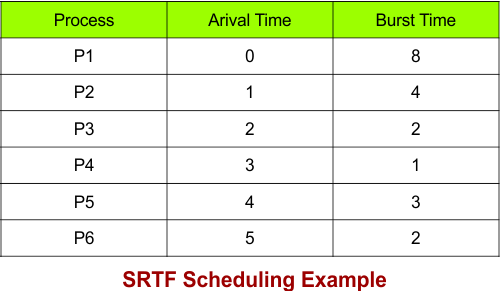
SRTF Scheduling Example 2
Consider the following table, which includes the Process, Arrival time, and burst time.
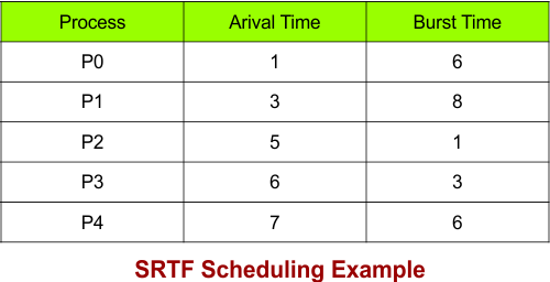
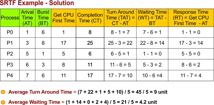
Gannt. Chart of the given example 2 is given below

The following diagram shows how to calculate the Completion Time (CT), Waiting Time (WT), Turnaround Time (TAT), Average Waiting Time (AWT), Average Turnaround Time (ATAT), and Response Time (RT) of example 4
SRTF Scheduling Example 3
Consider the following table, which includes the Process, Arrival time, and burst time.
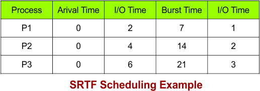
Gannt. Chart of the given example 3 is given below
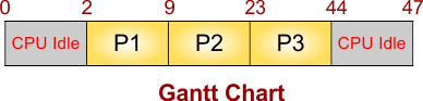
The following diagram shows how to calculate the Completion Time (CT), Waiting Time (WT), Turnaround Time (TAT), Average Waiting Time (AWT), Average Turnaround Time (ATAT), and Response Time (RT) of example 3
SRTF Scheduling Example 4
Consider the following table, which includes the Process, Arrival time, and burst time.
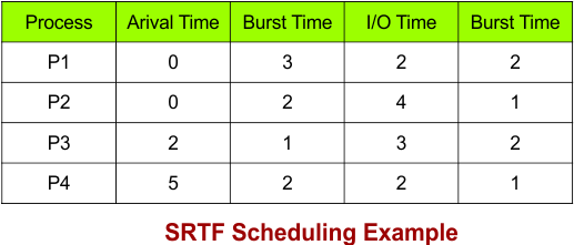
Gannt. Chart of the given example 4 is given below

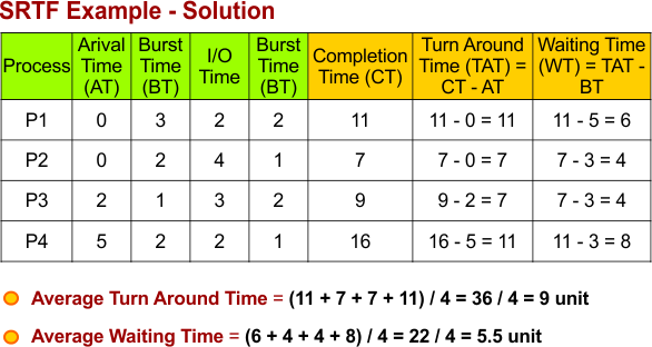
The following diagram shows how to calculate the Completion Time (CT), Waiting Time (WT), Turnaround Time (TAT), Average Waiting Time (AWT), Average Turnaround Time (ATAT), and Response Time (RT) of example 4.
SRTF Scheduling Example 5
Consider the following table, which includes the Process, Arrival time, and burst time.
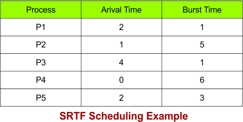
Gannt. Chart of the given example 5 is given below

The following diagram shows how to calculate the Completion Time (CT), Waiting Time (WT), Turnaround Time (TAT), Average Waiting Time (AWT), Average Turnaround Time (ATAT), and Response Time (RT).
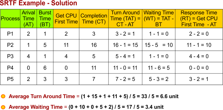
SRTF Scheduling Example 6
Consider the following table, which includes the Process, Arrival time, and burst time.
Gannt. Chart of the given example 6 is given below

The following diagram shows how to calculate the Completion Time (CT), Waiting Time (WT), Turnaround Time (TAT), Average Waiting Time (AWT), Average Turnaround Time (ATAT), and Response Time (RT).
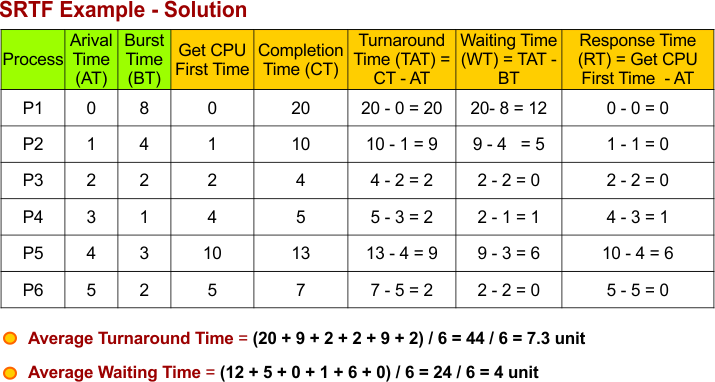
SRTF Scheduling Example 7
Consider the following table, which includes the Process, Arrival time, and burst time.
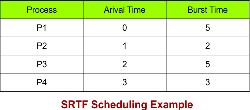
Gannt. Chart of the given example 7 is given below

The following diagram shows how to calculate the Completion Time (CT), Waiting Time (WT), Turnaround Time (TAT), Average Waiting Time (AWT), Average Turnaround Time (ATAT), and Response Time (RT) of example 7