Round Robin (RR) Scheduling in OS

Round Robin (RR) scheduling is one of the most popular CPU scheduling algorithms in OS. In Round Robin scheduling, each process gets a a CPU ofr fixed amount; this time is called a time quantum or time slice.

Once the time quantum is completed, the running process is preempted; it is moved to the end of the ready queue, and the next process from the ready queue is executed.

In this lecture, we will explain Round Robin (RR) scheduling with an example, its advantages, and disadvantages.

Round Robin (RR) Scheduling Working

Here is a simple working of Round Robin (RR) scheduling in an OS

• All processes which are ready to run are placed in the ready queue.  The first-come, first-served principle is applied to the ready queue by the CPU scheduler.
• Each process is executed by the CPU for a fixed unit of time, called a quantum period. For example, is quantom period is 2ms then each process can execute upto 2ms
• If any process completes its execution before or during the quantum period, it is simply removed from the ready queue. CPU moves to the next process.
• If the process still has work left after its time quantum ends, the CPU stops it for the moment. This is called preemption.
• The unfinished process goes to the end of the queue: The stopped process is placed at the back of the ready queue. This gives other processes a chance to use the CPU.
• The next process gets the CPU: The CPU now selects the next process from the front of the queue and gives it the same fixed amount of time.
• Processes get repeated turns: The CPU keeps moving through the queue. Each process gets a turn, and unfinished processes are moved to the back of the queue for another turn.
• The process continues until it finishes: A process may need several turns to complete. Every time it gets a turn, it uses the CPU for one time quantum until its work is finished.
• The process ends when the queue becomes empty: This cycle continues until all processes have completed their work. When no processes are left in the ready queue, the Round Robin scheduling is finished.

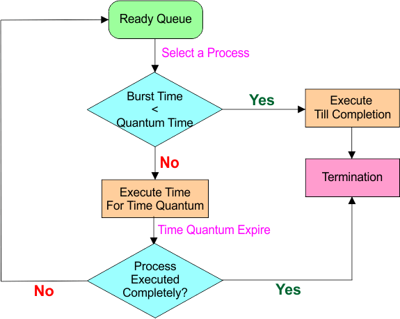
Round Robin (RR) Scheduling Flowchart

A flowchart of Round Robin (RR) scheduling in an OS is given below

Example of Round Robin (RR) Scheduling

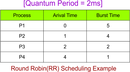
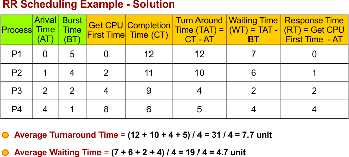
Consider there are four processes P1, P2, P3, and P4 with their arrival and burst times as shown in the following diagram, where the quantum period of each process is 2ms

Gantt Chart and Ready Queue Behaviour

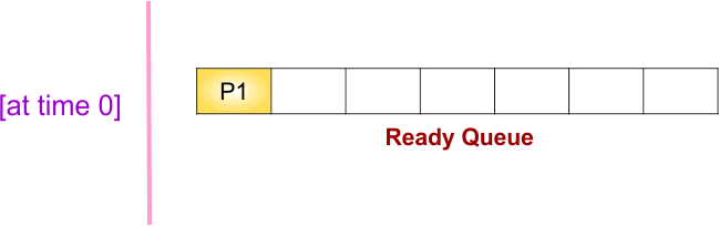
At time 0, only process P1 arrives, and it is placed in the ready queue. CPU will get P1 now, and the Gantt chart will start

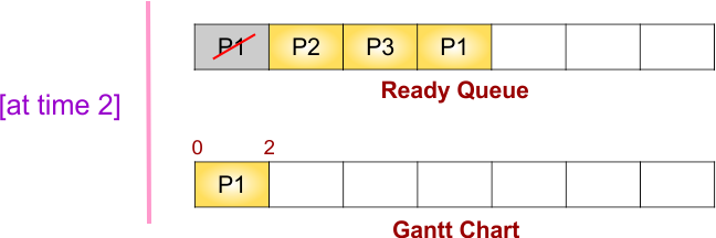
At time 0-2, P2 and P3 arrive, which are added to the end of the queue, and P1 is preempted after a quantum period of 2ms and added to the end of the ready queue. CPU now executes the next process in the ready queue, which is P2

At time 2-4, P4 arrives, which is added to the end of the queue, and P2 is preempted after a quantum period of 2ms and added to the end of the queue for its reminaing Burst Time (4ms – 2ms = 2ms). CPU now executes the next process in the ready queue, which is P3

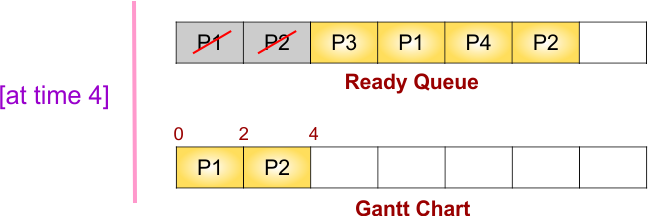
At time 4-6, no new process arrives, and P3 (having burst time of 2ms) completes its execution at time 6ms. CPU now executes the next process in the ready queue, which is P1

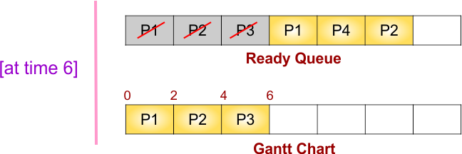
At time 6-8, no new process arrives, and P1 is preempted after a quantum period of 2ms and added to the end of the queue for its reminaing Burst Time (3ms – 2ms = 1ms). CPU now executes the next process in the ready queue, which is P4

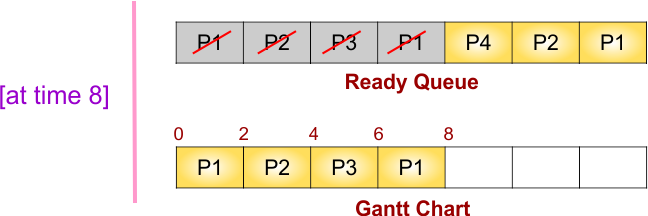
At time 8-9, no new process arrives, and P4 completes its execution at time 9ms. CPU now executes the next process in the ready queue, which is P2

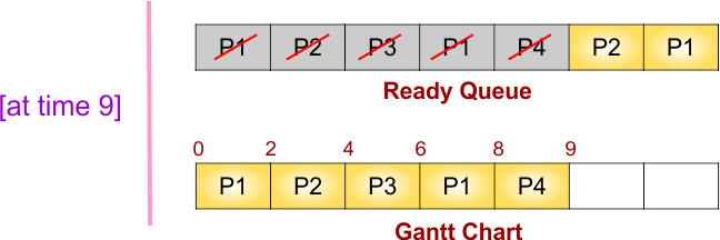
At time 9-11, no new process arrives, and P2 completes its execution at time 11ms. CPU now executes the next process in the ready queue, which is P1

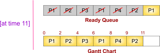
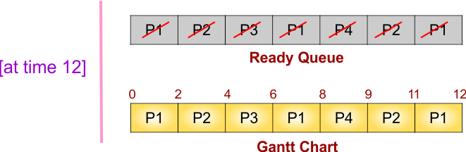
At time 11-12, no new process arrives, and P1 completes its execution at time 12ms. CPU now executes the next process in the ready queue; the ready queue is empty. That’s all

All calculations of the given example of RR are given below

Advantages of Round Robin (RR) Scheduling

Round Robin is a CPU scheduling algorithm in which each process gets a fixed amount of CPU time called a time quantum in a circular order. Here are the main advantages of Round Robin (RR) scheduling

1. Fairness: Every process gets an equal opportunity to use the CPU.
2. Good Response Time: Processes do not have to wait long to receive CPU time, making RR suitable for interactive systems.
3. Prevents Starvation: A process cannot be ignored indefinitely because every process gets its turn.
4. Simple to Implement: It is relatively easy to implement using a circular queue.
5. Suitable for Time-Sharing Systems: RR is especially useful when many users or processes need to share the CPU.
6. Better User Experience: Since processes regularly receive CPU time, the system feels more responsive.

In short, Round Robin provides fairness, prevents starvation, gives good response time, and is well suited for time-sharing and interactive operating systems.

Disadvantages of Round Robin (RR) Scheduling

Here are the main disadvantages of Round Robin (RR) scheduling

1. Higher Context Switching: If the time quantum is too small, the CPU spends a lot of time switching between processes.
2. Performance Depends on Time Quantum: Choosing an inappropriate time quantum can reduce system performance.
3. More Waiting Time: Processes may have to wait for several other processes to get their turns.
4. Higher Turnaround Time: Compared with some other scheduling algorithms, RR can result in a higher average turnaround time.
5. Not Ideal for Long CPU-Bound Processes: Long processes may require many rounds before completing.
6. Overhead: Frequent context switching creates additional CPU overhead.

In short, Round Robin can suffer from frequent context switching, higher waiting and turnaround times, and performance problems if the time quantum is not chosen properly.

Performance Parameters of Round Robin (RR) Scheduling

The main performance parameters used to evaluate Round Robin scheduling are:

CPU Utilization: Measures how efficiently the CPU is being used. RR generally aims for high CPU utilization.

Throughput: The number of processes completed by the CPU in a given period.

Turnaround Time: The total time taken from the submission of a process until its completion.

• Turnaround Time = Completion Time − Arrival Time

Waiting Time: The total time a process spends waiting in the ready queue.

• Waiting Time = Turnaround Time – Burst Time

Response Time: The time between submitting a process and the time it first gets CPU attention.

• Response Time = First CPU Start Time − Arrival Time

Context Switching Overhead: RR can have significant overhead because processes are frequently switched after each time quantum.

Effect of Time Quantum

The time quantum is very important in RR:

• Very small quantum: More context switches → higher overhead.
• Very large quantum: RR starts behaving like FCFS (First-Come, First-Served).
• Proper quantum: Provides a good balance between response time and overhead.

In short: The key performance parameters are CPU utilization, throughput, turnaround time, waiting time, response time, context-switching overhead, and fairness.