











Shortest Job First (SJF) Scheduling Examples
In the Shortest Job First (SJF) Scheduling in OS the CPU always executes the process with the shortest CPU burst time among all the processes available in the ready queue. This approach reduces the average waiting time and improves overall CPU performance.
In SJF Scheduling
- The process with the shortest CPU burst time is selected for execution first.
- If two or more processes have the same burst time, the process with the earlier arrival time is executed first.
- If both the arrival time and burst time are the same, the process with the smaller process ID (or lower order number) is executed first.
- SJF can be Non-Preemptive, where a running process continues until completion, or Preemptive (Shortest Remaining Time First – SRTF), where a newly arrived process with a shorter remaining burst time can interrupt the running process.
In this section, we will solve multiple Shortest Job First (SJF) Scheduling examples with Gantt charts, Completion Time (CT), Waiting Time (WT), Turnaround Time (TAT), Response Time (RT), Average Waiting Time (AWT), and Average Turnaround Time (ATAT). We will cover different scenarios, including same arrival time, different arrival times, non-preemptive SJF, preemptive SJF (SRTF), and examples involving I/O operations.
Formulas that will be used in this lecture are given below
|
SJF Scheduling Example: 01
Consider that there are 4 processes (P1, P2, P3, and P4) with their arrival and burst times, which are given in the following diagram
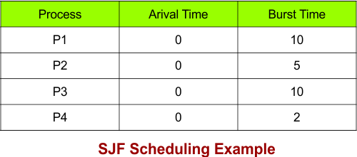
By using SJF scheduling, calculate completion time (CT), waiting time (WT), turnaround time (TAT), average waiting time (AWT), and average turnaround time (ATAT).
Solution
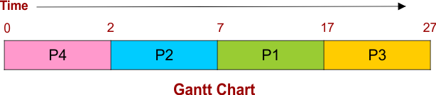
Gantt Chart of Example 1 is given below
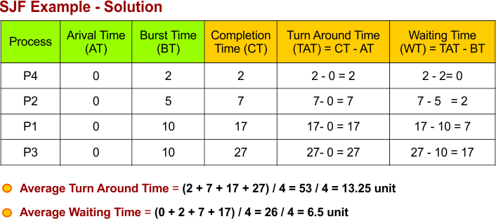
All Calculations
The following diagram calculates completion time (CT), waiting time (WT), turnaround time (TAT), average waiting time (AWT), and average turnaround time (ATAT).
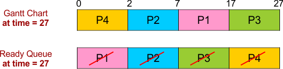
Ready Queue and Gantt Chart Behavior in Example 1
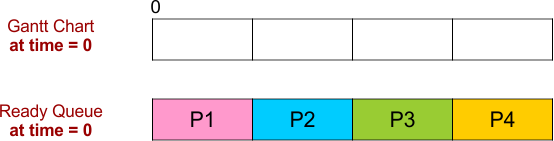
At time 0:
All processes (P1, P2, P3, and P4) enter the ready queue. The CPU scheduler compares their burst times (10, 5, 10, and 2). P4 has the shortest burst time (2 ms), so it is selected first.
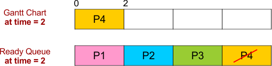
At time 2:
P4 completes its execution at time 2. The Ready Queue contains P1, P2, and P3, where P2 contains shortest burst time among P1, P2, and P3, so now it will be executed by the CPU.
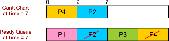
At time 7:
P2 completes its execution at time 7. The Ready Queue contains P1 and P3, where P1 and P2 contains similar burst time and arrival time. But P1 has smaller process ID, so now it will be executed by the CPU.
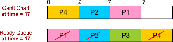
At time 17:
P3 completes its execution at time 17. The Ready Queue contains only P3, so now it will be executed by the CPU.
At time 27:
P3 completes its execution at time 27. The Ready Queue contains nothing. That’s all
SJF Scheduling Example: 02
Consider there are 5 processes (P1, P2, P3, P4, and P5) with their arrival and burst times, which are given in the following diagram
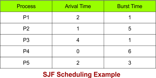
By using SJF scheduling, calculate completion time (CT), waiting time (WT), turnaround time (TAT), average waiting time (AWT), average turnaround time (ATAT), and response time (RT).
Solution
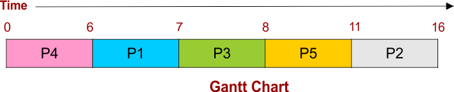
Gantt Chart of Example 2 is given below
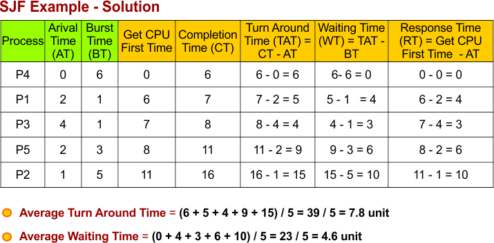
All Calculations
The following diagram calculates completion time (CT), waiting time (WT), turnaround time (TAT), average waiting time (AWT), average turnaround time (ATAT), and response time.
SJF Scheduling Example: 03
Consider there are 4 processes (P1, P2, P3, and P4) with their arrival and burst times, which are given in the following diagram
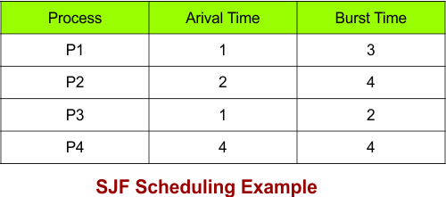
Using SJF scheduling, calculate the completion time (CT), waiting time (WT), turnaround time (TAT), average waiting time (AWT), and average turnaround time (ATAT).
Solution
Gantt chart for Example 3 is given below
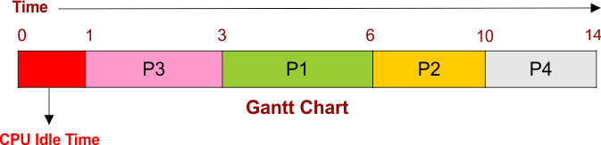
All Calculations
The following diagram calculates completion time (CT), waiting time (WT), turnaround time (TAT), average waiting time (AWT), and average turnaround time (ATAT).
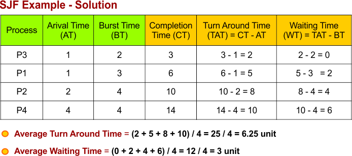
SJF Scheduling Example: 04
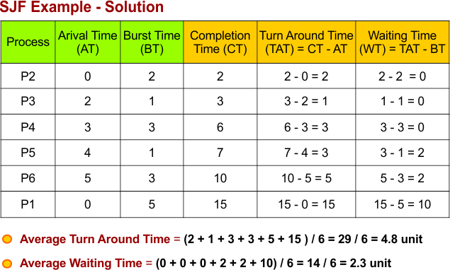
Consider there are 4 processes (P1, P2, P3, P4, P5 and P6) with their arrival and burst times, which are given in the following diagram
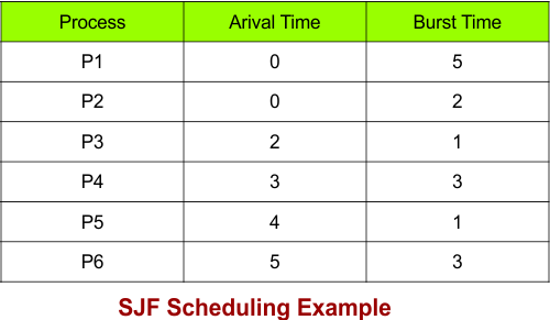
Using SJF scheduling, calculate the completion time (CT), waiting time (WT), turnaround time (TAT), average waiting time (AWT), and average turnaround time (ATAT).
Solution
Gantt chart for Example 4 is given below

All Calculations
The following diagram calculates completion time (CT), waiting time (WT), turnaround time (TAT), average waiting time (AWT), and average turnaround time (ATAT).
SJF Scheduling Example: 05
Consider there are 5 processes (P1, P2, P3, P4, and P5) with their arrival and burst times, which are given in the following diagram
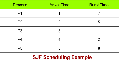
Using SJF scheduling, calculate the completion time (CT), waiting time (WT), turnaround time (TAT), average waiting time (AWT), and average turnaround time (ATAT).
Solution
Gantt chart for Example 5 is given below

All Calculations
The following diagram calculates completion time (CT), waiting time (WT), turnaround time (TAT), average waiting time (AWT), and average turnaround time (ATAT).