How to Calculate Average Waiting Time and Turnaround Time in CPU Scheduling

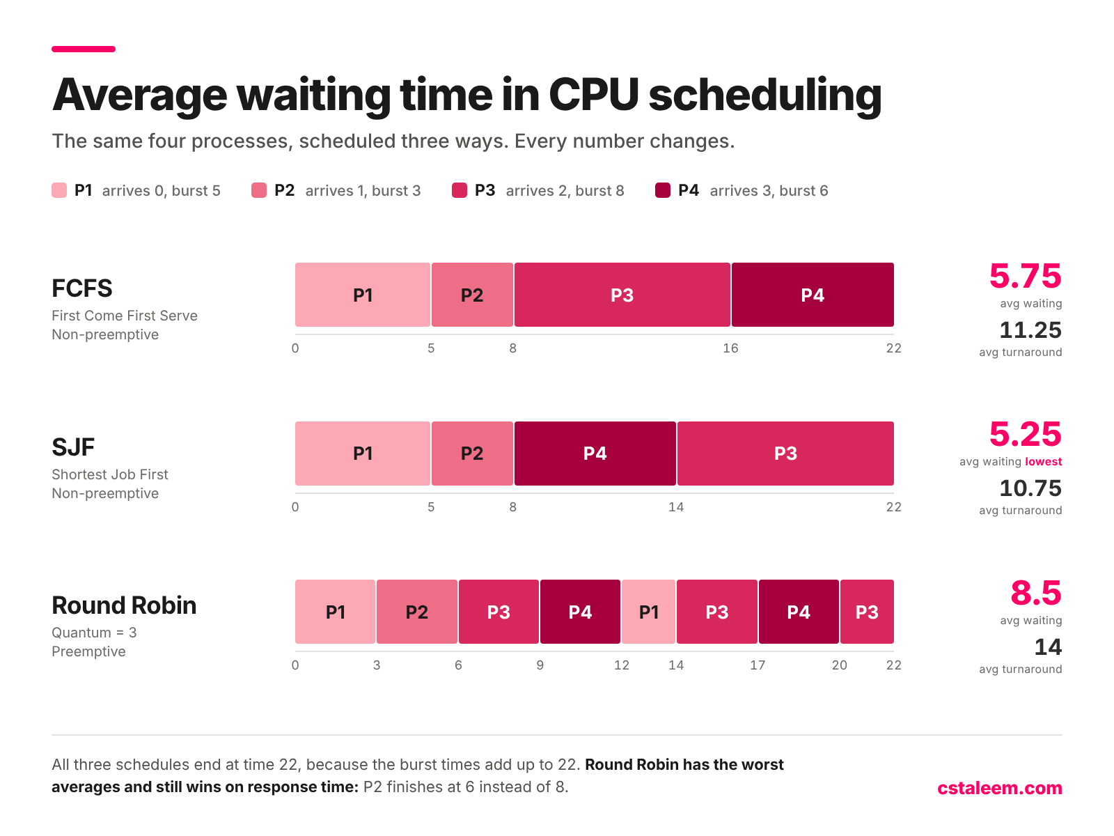
You have a table of processes with arrival times and burst times, and the question asks for the average waiting time. Two formulas get you there, and both work the same way in every scheduling algorithm:

Turnaround time = completion time – arrival time

Waiting time = turnaround time – burst time

Work out those two numbers for each process, add each column, divide by the number of processes. That is the whole method. The part that goes wrong is the schedule itself, because the completion times depend on which algorithm you are using, and a single misplaced time slice changes every number after it.

Below, the same four processes run through FCFS, non-preemptive SJF and Round Robin, with every step shown. The answers differ by a lot, which is the point.

The four times you need before you calculate anything

Arrival time is when the process enters the ready queue. It is given in the question.

Burst time is how long the process needs on the CPU. Also given.

Completion time is when the process finishes its last instruction. You read this off your Gantt chart, so it is the first thing you actually have to work out.

Turnaround time is the total time from arrival to completion, including every moment the process sat idle waiting its turn. Waiting time is that same span with the CPU time taken out.

If any of those four are still fuzzy, read the various times of a process first, because the rest of this will not stick without them. The definitions follow the standard ones used in Operating System Concepts, which is the textbook most university OS courses set.

The process set used in all three examples

Process	Arrival time	Burst time
P1	0	5
P2	1	3
P3	2	8
P4	3	6

Total burst time is 22 units. Keep that number. It is the fastest way to check your work later.

FCFS: run them in arrival order

First Come First Serve has no decision to make. Sort by arrival time and run each process to completion. P1 arrived first, so it goes first and nothing interrupts it.

Gantt chart:

P1: 0 to 5 | P2: 5 to 8 | P3: 8 to 16 | P4: 16 to 22

Process	Arrival	Burst	Completion	Turnaround	Waiting
P1	0	5	5	5	0
P2	1	3	8	7	4
P3	2	8	16	14	6
P4	3	6	22	19	13

Take P4 as the one worth reading twice. It arrived at 3 and finished at 22, so its turnaround time is 19. Subtract its 6 units of CPU time and it spent 13 units doing nothing but waiting. That happened because P3 needed 8 units and P4 was stuck behind it. This is the convoy effect, and it is the reason FCFS is taught first and used last.

Average turnaround time = (5 + 7 + 14 + 19) / 4 = 45 / 4 = 11.25

Average waiting time = (0 + 4 + 6 + 13) / 4 = 23 / 4 = 5.75

Four numbers you can add in your head. When the exam gives you ten or twelve processes, the arithmetic is where marks disappear, and pushing the column through a mean calculator catches the addition slip before you write the final answer.

SJF: pick the shortest burst that has arrived

Non-preemptive Shortest Job First looks at every process sitting in the ready queue and starts the one with the smallest burst time. Once a process starts, it finishes. The word to watch is arrived, because at any decision point you can only choose from processes whose arrival time has already passed.

Step through the decisions:

1. At t = 0, only P1 has arrived. Run P1 from 0 to 5.
2. At t = 5, P2 (3), P3 (8) and P4 (6) are all waiting. P2 is shortest. Run P2 from 5 to 8.
3. At t = 8, P3 (8) and P4 (6) remain. P4 is shorter. Run P4 from 8 to 14.
4. At t = 14, P3 is all that is left. Run P3 from 14 to 22.

Gantt chart:

P1: 0 to 5 | P2: 5 to 8 | P4: 8 to 14 | P3: 14 to 22

Process	Arrival	Burst	Completion	Turnaround	Waiting
P1	0	5	5	5	0
P2	1	3	8	7	4
P3	2	8	22	20	12
P4	3	6	14	11	5

Average turnaround time = (5 + 7 + 20 + 11) / 4 = 43 / 4 = 10.75

Average waiting time = (0 + 4 + 12 + 5) / 4 = 21 / 4 = 5.25

SJF beat FCFS by half a unit on average waiting time. On this small set the gap looks trivial. Swap P3’s burst to 20 and the gap widens fast, because SJF pushes the long job to the back where it can only delay itself.

That is also SJF’s problem. A process with a large burst time can keep getting passed over by shorter arrivals and never run, which is called starvation. Textbook questions rarely punish you for this, but you should name it if the question asks for a drawback.

One detail that gets skipped: a real scheduler does not scan the whole ready queue to find the shortest burst. It keeps the queue as a min-heap, so adding a process and pulling out the shortest both cost O(log n) rather than O(n). For a queue holding 1024 processes that is 10 steps instead of 1024, and you can confirm any figure like that with a log calculator set to base 2. The same O(log n) bound shows up across the asymptotic notations you use everywhere else in algorithms.

Round Robin with a 3 unit quantum

Round Robin gives every process a fixed slice of CPU time, then moves it to the back of the queue if it is not finished. It is preemptive, so a process can be stopped mid-execution, and that is what makes the trace harder to get right.

The rule that decides most exam answers: when a time slice ends, newly arrived processes join the queue before the process that was just preempted. Get this backwards and your chart will match the answer key for two slices and then diverge from everything after it.

Trace with quantum = 3:

Time	Running	Remaining burst after	Queue after the slice
0 to 3	P1	2	P2, P3, P4, P1
3 to 6	P2	0, done at 6	P3, P4, P1
6 to 9	P3	5	P4, P1, P3
9 to 12	P4	3	P1, P3, P4
12 to 14	P1	0, done at 14	P3, P4
14 to 17	P3	2	P4, P3
17 to 20	P4	0, done at 20	P3
20 to 22	P3	0, done at 22	empty

P1 only needed 2 more units in its second turn, so it ran 12 to 14 instead of taking the full quantum. A process never gets more than the quantum, but it can take less.

Process	Arrival	Burst	Completion	Turnaround	Waiting
P1	0	5	14	14	9
P2	1	3	6	5	2
P3	2	8	22	20	12
P4	3	6	20	17	11

Average turnaround time = (14 + 5 + 20 + 17) / 4 = 56 / 4 = 14

Average waiting time = (9 + 2 + 12 + 11) / 4 = 34 / 4 = 8.5

The three algorithms on the same data

Algorithm	Average waiting time	Average turnaround time
FCFS	5.75	11.25
SJF (non-preemptive)	5.25	10.75
Round Robin (q = 3)	8.5	14

Round Robin lost on both averages and it is still the one your operating system uses. Look at P2: it finished at time 6 under Round Robin against 8 under the other two, and the short interactive job is exactly the one a user notices. Round Robin trades average throughput for response time, which is why average waiting time on its own is a weak way to judge a scheduler.

The same arithmetic turns up again in disk scheduling, where you average seek times across a request queue instead of waiting times across a process queue. Different unit, identical calculation.

Where students lose marks

You computed waiting time as start time minus arrival time. This gives the right answer for FCFS and non-preemptive SJF, so it feels safe. It breaks in Round Robin, because a process waits several separate times. P1 starts at 0 and arrives at 0, which would give a waiting time of 0, when the real figure is 9. Always go through turnaround time.

You divided by the total burst time instead of the number of processes. The symptom is an average waiting time smaller than 1 on a question where individual waits were in double digits.

You ignored idle CPU time. If the earliest arrival is at t = 2, the CPU does nothing from 0 to 2 and every completion time shifts by 2. The schedule starts when the first process arrives, not at zero.

You put the preempted process ahead of a new arrival in Round Robin. At t = 3 in the example above, P4 arrives at exactly 3 and P1 is preempted at exactly 3. P4 goes in first. Reverse it and the whole trace after that point is wrong.

You broke an SJF tie by process number instead of arrival time. When two ready processes have equal burst times, the one that arrived earlier runs first. Check what your course notes say, because a few courses use process ID, and state your assumption in the answer either way.

Check your own answer in 20 seconds

Three checks will catch almost every arithmetic error.

The last completion time equals the sum of all burst times when the CPU never sits idle. Here the bursts add to 22, and all three schedules end at 22. If your chart ends at 21 or 23, a slice is the wrong width.

Average turnaround minus average waiting equals average burst time. The bursts average 22 / 4 = 5.5. Check each result: 11.25 – 5.75 = 5.5, 10.75 – 5.25 = 5.5, 14 – 8.5 = 5.5. All three pass. This check works on any process set and it catches a single wrong completion time instantly.

Non-preemptive SJF should never lose to FCFS on average waiting time for the same data. If your FCFS number comes out lower, one of the two schedules is wrong.

Frequently asked questions

What is the formula for average waiting time in CPU scheduling?

Add the waiting time of every process and divide by the number of processes. Each process waiting time is its turnaround time minus its burst time, and turnaround time is completion time minus arrival time.

Can the waiting time of a process be zero?

Yes. A process that starts as soon as it arrives and runs without interruption has a waiting time of zero. P1 in all the examples above is the usual case, since it arrives at t = 0 with an empty ready queue.

Why is average waiting time higher in Round Robin?

Every unfinished process goes to the back of the queue after its quantum, so long processes are interrupted repeatedly and accumulate waiting time in several separate stretches. What Round Robin buys in return is a shorter wait before each process runs for the first time.

Does turnaround time include waiting time?

Yes. Turnaround time is waiting time plus burst time, which is why subtracting the burst time from it gives you the waiting time.

How do you handle CPU idle time in the calculation?

Leave the gap in the Gantt chart and carry on. Idle time shifts the completion times of later processes, but the two formulas do not change. Waiting time counts only the time a process spent in the ready queue, so idle CPU before its arrival is not its wait.

Which scheduling algorithm gives the minimum average waiting time?

Shortest Job First is provably optimal for average waiting time on a fixed set of processes. It needs the burst times in advance, which a real operating system does not have, so schedulers estimate them instead.

What happens if the Round Robin quantum is very large or very small?

A quantum larger than the longest burst time turns Round Robin into FCFS, because no process is ever preempted. A very small quantum spreads CPU time evenly but spends more of it on context switching, so the useful work per second drops.