












Operating System Concepts You’ll Meet Again in Production: CPU, Memory and Processes
If you are studying operating systems, you have probably spent hours on CPU scheduling algorithms, process states, paging and disk scheduling. It is easy to see these topics as exam material that you will leave behind once you start building software.
They do not go away. Every server running in a data center or cloud account is managed by an operating system, and the people who keep those servers healthy watch numbers that come straight from the concepts in your syllabus. CPU utilization, load average, available memory, swap usage, process counts and I/O wait are all the OS reporting on its own scheduler, memory manager and I/O subsystem.
This article connects the two worlds. For each major OS topic, you will see which production metric it turns into, what that metric means, and what it tells an operations engineer when something goes wrong. The examples use Linux, because it runs a large share of the world’s servers and exposes these numbers clearly, but the ideas apply to any modern operating system.
Why Do OS Concepts Matter Once Software Is in Production?
OS concepts matter in production because almost every performance problem on a server is, underneath, a resource problem that the operating system is managing. When an application slows down, the cause is usually one of a small set of things: processes waiting for CPU time, memory running short, too many processes or threads, or storage that cannot keep up. Each of these is a topic from your OS course.
Operations teams rarely look at the scheduler or the page tables directly. Instead, they read metrics that the kernel publishes about its own work. On Linux, most of these come from the /proc filesystem, a virtual filesystem that exposes kernel data as readable files. Monitoring tools collect these values every few seconds, store them over time and raise alerts when they cross a threshold.
The map below shows how the main OS topics line up with the metrics you would see on a production dashboard. The rest of this article walks through each pair in turn.
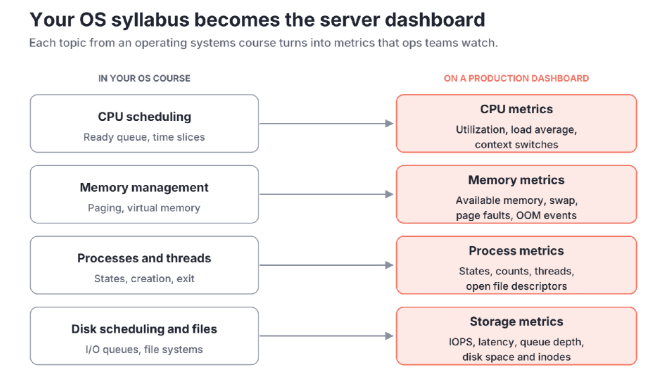
Image 1: Each topic in an OS course reappears as a set of metrics on a production dashboard.
If you understand the concept behind a metric, you can reason about what a strange number means instead of guessing. That skill separates engineers who can only read a dashboard from engineers who can explain it.
How Does CPU Scheduling Show Up in CPU Metrics?
CPU scheduling shows up in two kinds of metrics: how busy each CPU core is, and how many processes are waiting for a turn. In your OS course you learned that the scheduler picks which ready process runs next, and that processes not currently running wait in a ready queue. Production monitoring measures both sides of that picture.
CPU utilization is the share of time a core spends doing work rather than sitting idle. Linux splits it into categories that map neatly onto what you studied:
- User time is time spent running application code in user mode.
- System time is time spent in kernel mode, handling system calls, interrupts and scheduling itself.
- I/O wait is time the CPU sat idle while at least one process was waiting for disk I/O to finish.
- Steal time appears on virtual machines and shows time the hypervisor gave your virtual CPU’s turn to another guest.
High user time usually points to busy application code. High system time can suggest heavy system call activity or interrupt load. High I/O wait means the CPU is fine and the bottleneck is storage. Teams that do CPU usage monitoring look at this breakdown, not just the total, because the split tells you where to look next.
Load average is the ready queue made visible. It is the average number of processes that are running or ready to run over the last 1, 5 and 15 minutes. On Linux it also counts processes in uninterruptible sleep, which are usually waiting on disk. The number only makes sense next to the core count. A load of 4 on a 4-core server means every core is busy with nothing waiting. A load of 8 on the same server means, on average, four processes are queued for a turn.
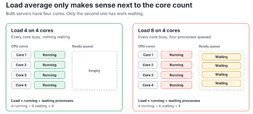
Image 2: Load average counts running and waiting processes, so read it against the number of cores.
Context switches count how often the scheduler swaps one process or thread off a core for another. Some switching is normal. A sudden jump can mean too many threads competing for too few cores, which wastes time on switching rather than useful work.
How Does Memory Management Show Up in Memory Metrics?
Memory management shows up as metrics for how much RAM is in use, how much can be freed when needed, and how often the system has to fall back on disk. The concepts are the ones from your paging and virtual memory chapters.
The first surprise for most students is that low free memory is usually not a problem. Linux uses spare RAM as a page cache, holding recently read file data so the next read is fast. That cache counts as used memory, but the kernel can drop it the moment an application needs the space. This is why monitoring tools focus on available memory, an estimate of how much memory could be given to new work without swapping. On Linux, it appears as MemAvailable in /proc/meminfo.
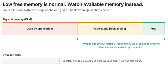
Image 3: Available memory includes page cache the kernel can reclaim, which is why free memory alone is misleading.
The other memory metrics follow directly from virtual memory theory:
- Swap usage shows how much memory has been moved out to disk. Some swap in use is not alarming on its own. Constant swapping in and out is a concern, because disk is far slower than RAM.
- Page faults count how often a process touches a page that is not currently mapped in RAM. Minor faults are resolved without disk access and are cheap. Major faults need a disk read and are expensive, so a rising major fault rate is an early warning of memory pressure.
- Out-of-memory events happen when the kernel cannot find memory at all. Linux then runs the OOM killer, which ends a process to free memory. In production, this usually looks like an application that suddenly restarted for no obvious reason.
When memory runs short, the system can enter thrashing, the state you studied where it spends more time moving pages between RAM and disk than doing useful work. On a dashboard, thrashing looks like low available memory, heavy swap activity, a rising major fault rate and high I/O wait, all at once.
How Do Processes and Threads Turn into Process Metrics?
Processes and threads turn into metrics that count them, track their states and measure what each one consumes. The process state diagram from your course is something operations engineers read every day, just in a different form.
On Linux, tools such as ps and top show each process with a one-letter state code:
- R (running or runnable) means the process is on a CPU or in the ready queue.
- S (sleeping) means it is waiting for an event, such as network data or a timer. Most processes spend most of their time here.
- D (uninterruptible sleep) means it is waiting on I/O and cannot be interrupted. Many D-state processes usually point to slow or stuck storage.
- Z (zombie) means the process has finished, but its parent has not yet collected its exit status. Zombies use almost no resources, but a growing count suggests a parent process with a bug.
Beyond states, process monitoring tracks how much CPU and memory each process uses, whether critical processes are running at all, and how many instances exist. A web server that should have eight worker processes but has none is an outage, even if the server’s overall CPU and memory look fine.
Two more counts are worth knowing. Thread count per process helps you spot thread leaks, where an application keeps creating threads and never releases them. Open file descriptors matter because Linux treats files, sockets and pipes as file descriptors, and each process has a limit. An application that hits that limit starts failing with errors such as “too many open files”, which is a classic production issue that traces straight back to OS fundamentals.
Effectively managing cybersecurity threats requires the establishment of a strong incident response plan, built around modern security incident response practices rather than a static document. This plan should also account for memory management and process monitoring, as unusual memory consumption, abnormal process activity, excessive resource utilization, and unauthorized processes can indicate potential security threats or system compromises.
How Does Disk I/O Show Up in Storage Metrics?
Disk I/O shows up as metrics for how much work storage is doing, how long each request takes and how many requests are waiting. In your course, disk scheduling algorithms decided the order in which queued requests were served. Production metrics measure the result of that queue.
The core storage metrics are:
- IOPS (input/output operations per second) shows how many read and write requests the disk handles.
- Throughput shows how much data moves per second, usually in megabytes.
- Latency (often called await on Linux) shows how long each request takes from submission to completion, including time spent queued.
- Queue depth shows how many requests are waiting or in progress. A queue that keeps growing means requests arrive faster than the disk can serve them.
- Utilization shows the share of time the device was busy. On modern SSDs and storage arrays that serve many requests in parallel, 100% utilization does not always mean the device is saturated, so read it alongside latency.
Latency is usually the metric that matters most to users. A disk can show modest IOPS and still make an application feel slow if each request takes too long.
Capacity is the other side of storage. Running out of disk space stops databases, breaks log writing and can bring down whole services. Linux file systems can also run out of inodes, the data structures that store file metadata, even when free space remains. That happens when an application creates millions of tiny files. Disk space monitoring watches both free space and growth rate, so teams can act before a disk fills rather than after.
How Do These Metrics Work Together When Troubleshooting?
These metrics work best when you check them in a fixed pattern rather than staring at every chart at once. One widely used pattern is the USE method, created by performance engineer Brendan Gregg. For every resource, it asks three questions:
- Utilization. How busy is the resource?
- Saturation. Is work queuing because the resource is full?
- Errors. Is the resource reporting failures?
The method works because it mirrors how an operating system manages resources. Each resource has a capacity, a queue for work that cannot be served yet, and ways to fail. Your OS course taught you all three for CPUs, memory and disks. The USE method simply turns them into a checklist.
Applied to a server, the checklist looks like the grid below. Saturation is often the most revealing column. A CPU at 70% utilization with a long run queue is in more trouble than a CPU at 95% with nothing waiting, because the queue is where users feel the delay.
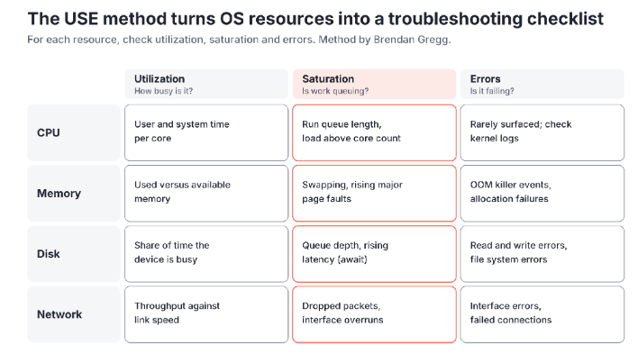
Image 4: The USE method applied to a server’s four main resources.
This is also how Linux server monitoring tools organize their dashboards: CPU, memory, disk and network panels, each showing how busy the resource is and whether work is backing up. Once you know the OS concept behind each panel, a production dashboard stops being a wall of numbers and becomes a set of questions you already know how to ask.
How Can You Practise Reading These Metrics as a Student?
You can practise on any Linux machine, including a virtual machine or a free cloud instance, using tools that ship with most distributions. Each one shows a part of the OS you have studied:
| Tool | What it shows | OS concept behind it |
|---|---|---|
| top or htop | Per-process CPU and memory, load average, process states | Scheduling, process states |
| vmstat 1 | Run queue, context switches, swap activity, CPU time split | Scheduling, virtual memory |
| free -h | Used, cached and available memory, swap | Paging, page cache |
| iostat -x 1 | IOPS, throughput, latency and utilization per disk | Disk scheduling, I/O queues |
| cat /proc/loadavg | Raw load averages and process counts | Ready queue |
| df -h and df -i | Disk space and inode usage | File systems |
A simple lab makes the connection stick. Open vmstat 1 in one terminal and start a CPU-heavy program in another, such as a loop that compresses a large file. Watch the run queue and user time rise. Then run a program that reads a large file from disk and watch I/O wait climb while user time stays low. Finally, start several memory-hungry processes and watch available memory fall and swap activity begin. Each experiment shows a chapter of your textbook happening live.
The skills you build this way carry straight into roles in DevOps, site reliability engineering and IT operations. Teams in those roles use observability platforms such as Motadata ObserveOps to collect these same metrics from hundreds of servers at once, but the questions they ask are the ones your OS course already prepared you to answer: what is busy, what is waiting, and what is failing.