Are Nested Loops Always Quadratic?

Two short Python programs can both contain nested loops, accept an input size of 100, and execute their innermost statement either 300 or 4,950 times. Counting the loop headers cannot explain that difference. To analyse nested loops, count how often the body runs, then ask how much work happens on each visit. Four familiar claims show where that reasoning can go wrong.

“Two nested loops mean quadratic time.”

A fixed inner limit breaks this rule immediately. Suppose a program makes three checks for each record. Here, n is the number of records, and visits counts executions of the innermost statement:

visits = 0

for row in range(n):

    for slot in range(3):

        visits += 1

For four records, the counter finishes at 12. For eight, it finishes at 24. There are always three visits per record, so the total is 3n. Doubling the input doubles the count. Under the usual introductory model of constant-cost counter updates and loop operations, this program has linear growth, written Θ(n).

The Greek letter theta describes a tight asymptotic growth bound. Big O describes an upper bound, which can be loose. Although a linear function also has a quadratic upper bound, calling this program “quadratic” misses its tighter linear behaviour. MIT’s lesson on Big O and theta develops that distinction.

What matters here is that three stays three as the input grows. If the inner limit were a second input, m, the visit count would instead be nm. You would need to state how the two input sizes relate before replacing them with a single variable.

The indentation has stayed the same; the growth has changed.

“Doing fewer comparisons makes the loop linear.”

Now consider comparing every record with the records before it. This avoids comparing a record with itself and avoids checking the same unordered pair twice:

visits = 0

for i in range(n):

    for j in range(i):

        visits += 1

With five records, the successive inner-loop counts are zero, one, two, three and four. The total is ten. The endpoint matters: Python’s definition of range excludes the stop value, so range(i) does not include i. Adding that extra visit on every row would count a different program.

For a positive integer input size, the total is the arithmetic series

C(n) = 0 + 1 + ··· + (n − 1) = n(n − 1) / 2.

You can derive it by writing the sequence forward and backward. Each paired column totals n − 1, and there are n columns. The paired rows contain twice the original sum, which explains the division by two. For an empty input, the loop performs zero visits and the closed formula also gives zero.

If that algebra is the sticking point, MathSolver accepts a typed problem and supports step-by-step explanations and follow-up questions. Enter the sum you obtained from the code and ask why its endpoints produce that formula. Then check the explanation against the five-record trace. The site warns that its answers can be wrong; a convincing derivation of the wrong sum would still describe the wrong loop.

The saving is real, but the growth remains quadratic: Θ(n2). Running this counter gives 4,950 visits for 100 records and 19,900 for 200. That is slightly more than four times as many, approaching a factor of four as the input grows. “Roughly half as many comparisons” and “a lower order of growth” are different claims.

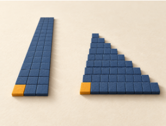
The triangular pattern shows why: removing half a square still leaves an area whose size depends on both dimensions.

“One line inside the loop is one unit of work.”

A line of code can hide a traversal. Initialize total = 0 before the loops, then replace the counter update with total += sum(values), where values contains n ordinary numbers and remains unchanged. Each visit now includes a pass through that collection. Python documents sum as summing the items of an iterable; its short name does not make the traversal disappear.

In the three-checks-per-record example, a linear number of visits would each perform a linear amount of work. Under constant-cost arithmetic, that makes the total quadratic. In the pair-comparison example, the same replacement would make the total cubic. Before assigning a complexity class, inspect the called operation as carefully as the loop bounds.

There is a practical repair when the collection really stays unchanged. Compute its sum once. Store the result, then reuse it inside the loop. This removes repeated calculation. It would not be a valid substitution if the collection changed between visits and the program needed the updated sum each time.

Try explaining that condition without looking at the code. Then change just one detail: the collection now gains an item on every outer iteration. Would the same repair still return the intended result? A useful practice question changes an assumption, forcing you to check the reasoning behind the label.

Keep the model visible too. These examples treat arithmetic on the values as constant-cost work. Very large integers, expensive comparisons, file access or network requests require a more detailed account. “One visit” is a unit you chose for analysis, not a promise about everything the program might do.

“You still need to measure the running program.”

This claim holds. Growth describes how work scales; timing measures a particular implementation and environment. Two quadratic implementations can have very different runtimes at the input sizes an application actually receives.

Separate counting from timing. Keep counters and small traces while checking the analysis, then remove diagnostic printing before measuring speed. Choose inputs for the case you described: a search that exits on its first comparison cannot validate its worst-case runtime.

Python’s timeit documentation recommends repeated measurements because other programs can interfere. It treats the minimum as a possible lower bound for that snippet on that machine, while advising inspection of all readings. Exclude setup when it falls outside the operation you intend to measure.

Record input sizes, the operation timed and the Python version. Measurements can expose a mistaken model, but a close fit at a few sizes is not proof of the formula.

When an analysis and a measurement disagree, return to the body of the loop. The missing cost may be sitting inside a single function call.