


Segmentation in Operating System
Segmentation is a memory management technique in operating systems where a process is divided into variable-sized logical segments, based on the functionality of the program. Common segments include:
-
Code segment (instructions of the program),
-
Data segment (global variables, constants),
-
Stack segment (function calls, return addresses, local variables)
-
Heap segment (dynamic memory)
Unlike paging, which divides the process memory into equal fixed-size blocks (pages), segmentation divides memory into logical units of variable sizes. This makes segmentation closer to the way programmers think about memory (functions, variables, objects, etc.), while paging is hardware-focused and uniform.
Note: When a program is executed, it becomes a process. The operating system loads the program into RAM. Under segmentation, instead of loading the entire program as one continuous block, it is divided into segments, and each segment is loaded into available memory locations.
Need of Segmentation in OS
Segmentation is needed in an OS because it provides logical division of a program, which makes memory management closer to how users and programmers think about their code. Unlike paging, which simply divides memory into fixed-size pages for the benefit of the OS, segmentation organizes memory into meaningful units such as functions, procedures, and data structures.
Why Paging Alone is Not Enough
In paging, a process is broken into equal-sized pages. These pages can scatter across memory.
-
Example: Suppose there is an Add() function. Paging may split this function into two pages, say Page 3 and Page 4.
-
If the CPU is executing Page 3 and a page fault occurs, Page 4 might be swapped out of memory. This means the Add() function cannot execute fully, lowering efficiency and performance.
How Segmentation Solves the Problem
In segmentation, each segment contains a complete logical unit, like the entire main() function, Add() function, or a full data structure.
-
This ensures that a function or data block is kept together in memory.
-
When a segment is loaded, the entire function is available to the CPU, avoiding the issue of incomplete execution.
Types of Segmentation in Operating Systems
Segmentation has various types in operating systems, which depend on how memory is organized and accessed. The most important types are given below
1. Fixed-Size Segmentation
Fixed-size segmentation is a memory management technique where a process is divided into segments of equal, fixed size. The operating system allocates memory in fixed-size blocks for each segment, simplifying memory management by ensuring that each segment is handled consistently. This approach is particularly useful in systems where memory requirements are relatively predictable, but it comes with certain trade-offs in terms of efficiency.
While the fixed-size approach reduces external fragmentation (unused gaps in memory), it often leads to internal fragmentation when the allocated memory does not perfectly match the process’s needs. This results in wasted memory within segments, making fixed-size segmentation less efficient when processes require smaller or varying amounts of memory.
Example of Fixed-Size Segmentation
Considering fixed-size segmentation, where:
- Total memory required by the process: 10 KB
- Fixed size of each segment: 4 KB
- The process will be divided into 3 segments of 4 KB each, leading to a total allocation of 12 KB (3 * 4 KB).
For First Segment (Data):
- Allocated memory: 4 KB
- Memory required by the process: 3 KB
- Internal fragmentation: 4 KB (allocated) – 3 KB (used) = 1 KB of unused memory.
- Result: 1 KB of internal fragmentation occurs in the first segment.
For Second Segment (Code):
- Allocated memory: 4 KB
- Memory required by the process: 2.5 KB
- Internal fragmentation: 4 KB (allocated) – 2.5 KB (used) = 1.5 KB of unused memory.
- Result: 1.5 KB of internal fragmentation occurs in the second segment.
For Third Segment (Stack):
- Allocated memory: 4 KB
- Memory required by the process: 3.5 KB
- Internal fragmentation: 4 KB (allocated) – 3.5 KB (used) = 0.5 KB of unused memory.
- Result: 0.5 KB of internal fragmentation occurs in the third segment.
Diagram Example of Memory Allocation:
 Used In:
Fixed-size segmentation is commonly applied in real-time embedded systems and real-time operating systems (RTOS). These systems often have predictable and static memory requirements, such as in robotic controllers, automotive systems, or industrial equipment, where memory needs are well-defined. For example, a robotic controller running a real-time OS might use fixed-sized memory blocks (e.g., 4 KB per segment) to allocate memory for critical tasks, ensuring predictable and reliable performance.
Advantages:
-
No or Mininal External Fragmentation: In Fixed-Sized Segmentation, because the memory is divided into fixed-size blocks (e.g., 4 KB each), external fragmentation is minimized or eliminated.
-
When memory is allocated, it always takes up one or more whole fixed-size blocks. This means there are no small gaps between allocated blocks that cannot be used (which is what causes external fragmentation).
-
- Simplified Memory Management: The use of fixed-size segments makes memory allocation straightforward because each segment is the same size. This simplicity reduces the overhead of complex memory management schemes.
Disadvantages:
-
Internal Fragmentation: When the required memory for a process is less than the allocated segment size, the unused portion within the segment results in wasted space. For example, if a process only needs 3 KB, but the segment is 4 KB, 1 KB of internal fragmentation occurs.
2. Variable-Sized Segmentation (Pure Segmentation)
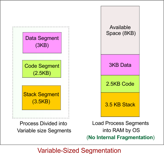
Variable-sized segmentation (also known as pure segmentation) is a memory management technique where a process is divided into segments of varying sizes, depending on the specific needs of each segment. Unlike fixed-size segmentation, where each segment has a predetermined, equal size, variable-sized segmentation allows the size of each segment to change dynamically to match the exact memory requirements of the process.
This approach is particularly useful for processes with different types of data, such as code, data, and stack, where each type may have different memory needs. However, it comes with its own set of challenges, particularly with regard to memory fragmentation.
Example of Variable-Sized Segmentation
Let’s consider a process that requires 10 KB of memory but uses variable-sized segments for different parts of the process (e.g., code, data, and stack). The process will be divided into 3 segments, but their sizes will vary depending on the requirements of each part. Here are the segment sizes:
- Segment 1 (Data): 3 KB
- Segment 2 (Code): 2.5 KB
- Segment 3 (Stack): 3.5 KB
In this case, no internal fragmentation occurs for any segment because the segments are sized exactly to the process’s needs (there’s no wasted space within each segment).
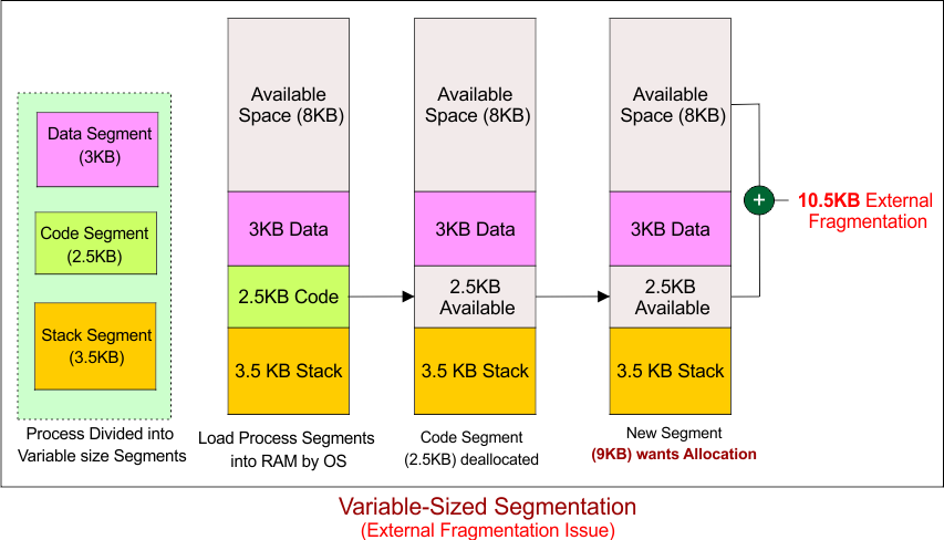
Now, Let’s Assume Segment 2 is Removed (Deallocated). After Segment 2 (Code) is deallocated. Next, Let’s Try to Allocate a 9 KB Segment:
There is a total of 10.5 KB of free space available:
-
8 KB of free space
-
2.5 KB free space (from deallocated Segment 2).
However, the free space is scattered into smaller blocks. There is no single block of 9 KB available, even though there’s 10.5 KB of free space in total. This is an example of External Fragmentation.
External Fragmentation Explanation
-
External Fragmentation happens because the free memory is not contiguous; it’s split into smaller blocks that cannot be used together.
-
In this case, even though there’s enough total free memory (10.5 KB), the free blocks (8 KB and 2.5 KB) cannot fit the new 9 KB segment because they are not contiguous.
Used In:
Variable-sized segmentation is commonly used in systems where memory needs are dynamic and variable. This approach is often found in general-purpose operating systems (e.g., UNIX, Windows) or systems that manage processes with different memory requirements, such as code, data, and stack segments. It’s also used in systems with complex tasks or multi-tasking environments, where processes have different requirements for each part of their execution.
Example: A general-purpose operating system like Linux might divide a process into segments where the code (e.g., executable instructions) might need more memory than the stack (e.g., temporary variables). These segments will be allocated memory according to their exact size requirements.
Advantages:
-
Flexible Memory Allocation: Variable-sized segmentation allows the system to allocate memory in precise amounts, minimizing wasted space. Each segment is sized to match the specific needs of that segment, making it highly adaptable.
-
Efficient Memory Usage: Since each segment is sized according to the process’s requirements, internal fragmentation is minimized, as there is no unused memory within each segment.
Disadvantages:
-
External Fragmentation: The main issue with variable-sized segmentation is external fragmentation. As segments of different sizes are allocated and deallocated, free memory in the system may become fragmented, leaving small gaps between segments that cannot be utilized effectively.
-
Complex Memory Management: Managing variable-sized segments can be more complex compared to fixed-size segments. The operating system needs to track varying segment sizes and their allocation, which increases the overhead of memory management.
3. Virtual Memory Segmentation
Virtual Memory Segmentation is a memory management technique used in modern operating systems that allows a program to be divided into multiple segments, where only the necessary segments are loaded into RAM (Random Access Memory) at any given time. It combines the advantages of segmentation (division of a program into logical parts like code, data, stack, etc.) and virtual memory (using disk space to extend the available RAM). This method allows the system to handle large programs and processes, even if the physical memory is not large enough to hold the entire program.
How Virtual Memory Segmentation Works:
-
Segmentation: A process is divided into multiple segments, each of which can grow or shrink dynamically during runtime (e.g., code segment, data segment, stack segment).
-
Virtual Memory: The system provides each process with the illusion of having contiguous memory by using a combination of physical RAM and disk storage. Only the parts of the program that are actively in use (the “demanded” segments) are loaded into RAM.
-
Demand Paging: When a process needs a segment that is not in memory, a page fault occurs, and the operating system loads the required segment from the disk into RAM. This is called demand paging, where only the necessary parts of the process are swapped in and out of memory as needed.
-
Segmentation with Virtual Memory: Each segment (e.g., code segment, data segment) is treated as a unit that can be swapped between RAM and disk. The operating system tracks the location of each segment, ensuring that the program runs smoothly without needing all of its segments in memory simultaneously.
Example of Virtual Memory Segmentation:
Let’s say a process needs 12 KB of memory in total, but only 6 KB can be loaded into physical memory at a time. The process is divided into 3 segments, each of 4 KB, but only the segments actively being used are loaded into RAM.
-
Total memory required by the process: 12 KB
-
Physical memory available: 6 KB
-
Segments:
-
Segment 1 (Code): 4 KB
-
Segment 2 (Data): 4 KB
-
Segment 3 (Stack): 4 KB
-
The operating system will load Segment 1 (Code) and Segment 2 (Data) into RAM. When the process needs access to Segment 3 (Stack), it will cause a page fault, and the operating system will swap Segment 1 or Segment 2 out of RAM and load Segment 3 from disk.
Diagram Example of Virtual Memory Segmentation:
| Segment 1 (4 KB) | Segment 2 (4 KB) | Segment 3 (4 KB) |
| (Code – In RAM) | (Data – In RAM) | (Stack – In Disk) |
+——————-+——————-+——————-+
| RAM | RAM | Disk |
+——————-+——————-+——————-+
-
Segment 1 (Code) and Segment 2 (Data) are in RAM.
-
Segment 3 (Stack) is not in RAM and resides in Disk.
-
When the program accesses Segment 3, the operating system swaps it into RAM from the disk.
Used In:
Virtual memory segmentation is widely used in modern operating systems like Windows, Linux, and macOS. It allows these systems to handle large applications and multitasking environments where the total memory required by the system exceeds the physical memory capacity. For example, large programs like web browsers or data analysis software require the use of virtual memory to run effectively even on machines with limited physical memory.
Advantages:
-
Efficient Memory Usage:
Only the segments that are actively being used are loaded into RAM, which allows more programs to run simultaneously, even if they require more memory than what is physically available. -
Isolation Between Processes:
Each process is given the illusion of having its own contiguous memory. This provides isolation and prevents one process from directly accessing or interfering with the memory of another process. -
Larger Programs:
Virtual memory allows systems to run larger programs than would otherwise fit into physical RAM, as the system can swap segments in and out of RAM as needed. -
Simplified Programming Model:
Developers can write programs as if they have access to a large, continuous block of memory, without worrying about physical memory limitations.
Disadvantages:
-
Page Fault Overhead:
When a segment is not in RAM and needs to be swapped in, it causes a page fault, which can slow down the system if it happens frequently. -
Increased Complexity:
Managing virtual memory with segmentation increases the complexity of the operating system. The system must track the location of all segments and handle swapping efficiently. -
Slower Performance:
While virtual memory allows large programs to run, disk I/O (swapping data between RAM and disk) is much slower than accessing memory directly, leading to potential performance degradation when the system is under heavy load.
4. Segmented Paging (Hybrid Approach)
Segmented Paging is a hybrid memory management technique that combines both segmentation and paging to take advantage of the strengths of each method while minimizing their respective weaknesses. This approach divides a process into segments, each of which is further divided into pages of fixed size. By combining the flexibility of segmentation (which allows the program to be divided into logical parts) with the efficiency of paging (which ensures that memory is divided into fixed-sized blocks), segmented paging helps in better memory management, especially for larger programs.
How Segmented Paging Works:
-
Segmentation: The process is divided into logical segments, such as the code segment, data segment, and stack segment. Each segment can grow or shrink dynamically based on the program’s needs.
-
Paging: Each segment is then divided into fixed-size pages (for example, 4 KB per page). This ensures that memory is allocated in smaller, manageable units, making it easier to load parts of a process into memory without the need for contiguous memory allocation.
-
Page Table for Each Segment: For each segment, there is a page table that stores the mapping between the logical pages and physical frames in RAM. This allows the operating system to efficiently manage memory by mapping logical addresses to physical addresses.
-
Segment Table: The segment table stores the base address of each segment’s page table, so the operating system knows where to find the page tables for each segment.
Example of Segmented Paging:
Let’s say a process requires 12 KB of memory and is divided into 3 segments, each of 4 KB. Each segment is then divided into pages of 4 KB each. So, the process will have 3 segments and 3 pages.
-
Total memory required: 12 KB
-
Segment 1 (Code): 4 KB
-
Segment 2 (Data): 4 KB
-
Segment 3 (Stack): 4 KB
Each segment is broken into 1 page (because each page is 4 KB). The system uses segment tables and page tables to map the segments and pages to physical memory.
Memory Allocation Breakdown:
1. Segment 1 (Code):
-
Allocated memory: 4 KB
-
Page Table: Maps the 4 KB code segment into physical memory.
-
Result: Code segment is divided into pages (in this case, only 1 page of 4 KB) and mapped to physical frames.
2. Segment 2 (Data):
-
Allocated memory: 4 KB
-
Page Table: Maps the 4 KB data segment into physical memory.
-
Result: Data segment is divided into pages and mapped to physical frames.
3. Segment 3 (Stack):
-
Allocated memory: 4 KB
-
Page Table: Maps the 4 KB stack segment into physical memory.
-
Result: Stack segment is divided into pages and mapped to physical frames.
Diagram Example of Segmented Paging:
| Segment 1 (Code) | Segment 2 (Data) | Segment 3 (Stack) |
| Page 1 (4 KB) | Page 1 (4 KB) | Page 1 (4 KB) |
| (In RAM) | (In RAM) | (In RAM) |
+——————-+——————-+——————-+
-
Each segment is divided into pages, and each page is mapped to a physical memory frame.
-
The segment table keeps track of the starting address for each segment, while the page table maps the pages to physical frames in RAM.
Used In:
Segmented Paging is commonly used in modern operating systems like Linux and Windows, where it offers the flexibility of segmentation combined with the efficient memory management provided by paging. This method is ideal for systems that need to handle large and complex programs, as it efficiently manages both the logical division of programs and the physical allocation of memory.
Advantages:
-
Combines Flexibility and Efficiency:
-
Segmentation provides logical organization of memory, while paging ensures that memory is allocated in fixed-size blocks, reducing the risks of fragmentation.
-
-
Reduces External Fragmentation:
-
Since pages are of fixed size, the risk of external fragmentation (gaps between memory allocations) is minimized.
-
-
Improved Memory Utilization:
-
The system only loads the required pages of a segment into RAM, making it possible to handle larger programs efficiently, even when physical memory is limited.
-
-
Better Performance for Multitasking:
-
Segmented paging allows the operating system to allocate memory more efficiently for multiple processes running simultaneously.
-
Disadvantages:
-
Complex Memory Management:
-
The combination of segment tables and page tables increases the complexity of memory management. The operating system must track both the logical segments and the physical memory frames for each page.
-
-
Overhead in Accessing Memory:
-
With multiple levels of mapping (segment table and page table), accessing memory involves extra lookups and translations, leading to higher overhead compared to simpler memory management techniques.
-
-
Fragmentation within Segments:
-
While external fragmentation is reduced, internal fragmentation can still occur if the last page of a segment is not fully utilized, especially if the segment size doesn’t align perfectly with page boundaries.
-
5. Shared Segmentation
Shared Segmentation is a memory management technique that allows multiple processes to share the same segment of memory. Instead of each process having its own copy of a segment (such as a shared library or common data), shared segmentation enables multiple processes to access and modify a common segment of memory. This technique is commonly used for efficient memory usage in cases where certain parts of a program or data are used by multiple processes simultaneously.
How Shared Segmentation Works:
-
Segment Division:
A process is divided into logical segments, such as code, data, and stack. Some segments, particularly those that are used by multiple processes (e.g., libraries or data), are marked as shared segments. -
Shared Memory:
The shared segment is mapped to the same physical memory location for multiple processes. Instead of having separate copies of the segment in each process’s memory, the operating system ensures that all processes access the same memory block for shared data. -
Permissions:
Each shared segment has access control permissions, such as read-only or read-write. These permissions control how processes can interact with the shared memory. For example, shared libraries might be marked as read-only to prevent multiple processes from modifying them. -
Segment Tables:
Each process has its own segment table that tracks the base address and size of its segments. For shared segments, the segment table entry will point to the same physical memory location for all processes that use the shared segment. -
Synchronization:
Processes that share a segment must typically use some form of synchronization to avoid conflicts (e.g., using locks or semaphores). If two processes try to modify the shared segment simultaneously, this can lead to data corruption or inconsistencies.
Example of Shared Segmentation:
Consider three processes running on a system, all of which need to access a common data segment (e.g., a shared configuration file or database). Instead of loading three separate copies of the data into memory, the operating system allocates one shared segment that all processes can access.
-
Process 1: Reads the shared data.
-
Process 2: Modifies the shared data.
-
Process 3: Also reads and writes to the shared data.
The operating system ensures that all three processes access the same physical memory for the shared segment, reducing memory usage and enabling efficient communication between processes.
Memory Allocation Breakdown:
1. Shared Segment (Data):
-
Allocated memory: 4 KB
-
Memory required by the processes: 4 KB
-
Internal fragmentation: 0 KB (since all processes use the memory efficiently)
-
Result: Multiple processes share the same physical memory for the data segment.
2. Non-Shared Segment (Code):
-
Each process will have its own code segment (not shared). This segment will be allocated separately in each process’s memory.
Diagram Example of Shared Segmentation:
| +——————-+——————-+——————-+ | Process 1 | Process 2 | Process 3 | | (Code – Private) | (Code – Private) | (Code – Private) | | 4 KB (Used) | 4 KB (Used) | 4 KB (Used) | +——————-+——————-+——————-+ | Shared Data Segment (4 KB) Shared by all Processes | | 4 KB (Used) | | (In RAM) | +——————————————————-+ |
-
Shared Data Segment (4 KB) is mapped into the same physical memory for all three processes.
-
Code segments are private and specific to each process.
Used In:
Shared segmentation is commonly used in multi-process systems where certain data, such as shared libraries, configuration files, or common databases, need to be accessed by multiple processes. Shared memory is often used for inter-process communication (IPC), allowing processes to exchange data efficiently. This technique is commonly seen in systems like Linux, UNIX, and Windows when sharing common resources between processes.
Advantages:
-
Efficient Memory Usage:
By allowing multiple processes to share a single copy of the segment, shared segmentation helps reduce memory usage. This is particularly useful for read-only data (e.g., libraries) that don’t need to be modified by each process. -
Faster Communication Between Processes:
Shared memory provides a fast method of communication between processes since they can directly read from and write to the same memory location, avoiding the overhead of inter-process communication mechanisms like message passing or file systems. -
Reduced Redundancy:
Shared segments eliminate the need to duplicate data across multiple processes, reducing redundancy and saving memory space.
Disadvantages:
-
Security and Access Control:
Since multiple processes access the same memory, there is a risk of unauthorized access or data corruption if proper access control mechanisms are not implemented. Permissions must be carefully managed to ensure that only authorized processes can modify the shared data. -
Synchronization Issues:
Shared segments often require synchronization (e.g., locks or semaphores) to prevent multiple processes from accessing or modifying the shared data at the same time. Improper synchronization can lead to data inconsistencies or crashes. -
External Fragmentation:
Although shared memory reduces internal fragmentation within each segment, external fragmentation can occur over time as segments are allocated and deallocated, leading to inefficient use of physical memory.
6. Dynamic Segmentation
Dynamic Segmentation is a memory management technique where the size of the segments can grow or shrink dynamically during the runtime of a process. Unlike fixed-size segmentation, where each segment has a pre-defined size, dynamic segmentation allows segments to adjust in size according to the needs of the process, based on the data it is processing and the operations it is performing.
In this approach, a process is still divided into logical segments, such as code, data, and stack, but each segment can change its size during execution. This makes dynamic segmentation more flexible and efficient for managing memory compared to fixed-size systems, especially when the memory requirements of a process vary over time.
How Dynamic Segmentation Works:
-
Segment Table:
Each process has a segment table that holds the base address and size of each segment. As the process runs, the size of each segment can be modified dynamically based on the memory requirements of the process. -
Memory Allocation:
The operating system allocates memory to segments as needed. If a segment grows, the operating system allocates more memory to that segment, expanding it. Similarly, if a segment shrinks, memory is released. -
Segment Swapping:
The operating system can swap entire segments in and out of physical memory as needed. If a segment grows beyond the available physical memory, it may be swapped to disk until needed again. -
Fragmentation:
While internal fragmentation (unused space within a segment) is minimized, external fragmentation (unused gaps between segments) can occur, especially if segments are not contiguous.
Example of Dynamic Segmentation:
Let’s consider a process that requires memory for different segments, but the sizes of these segments vary as the process runs.
-
Total memory required initially: 8 KB
-
Initial segment sizes:
-
Code segment: 4 KB
-
Data segment: 3 KB
-
Stack segment: 1 KB
-
During execution, if the data segment grows due to large inputs or calculations, the operating system dynamically allocates additional memory. Similarly, if the stack segment shrinks, memory is released.
-
After some time:
-
The Data segment grows to 5 KB (from 3 KB).
-
The Stack segment shrinks to 0.5 KB (from 1 KB).
-
The Code segment remains unchanged.
-
Diagram Example of Dynamic Segmentation:
| +——————-+——————-+——————-+ | Segment 1 (Code) | Segment 2 (Data) | Segment 3 (Stack) | | 4 KB (Used) | 5 KB (Used) | 0.5 KB (Used) | | (Base: 0) | (Base: 4) | (Base: 9) | +——————-+——————-+——————-+ |
-
The Code segment (4 KB) starts at address 0.
-
The Data segment (5 KB) starts at address 4 (just after the code segment).
-
The Stack segment (0.5 KB) starts at address 9, but it could shrink or grow during execution.
Used In:
Dynamic segmentation is used in modern operating systems like UNIX and Linux for multitasking and multi-user environments, where memory needs can change dynamically based on the execution of different processes. It is also found in systems with large, complex programs, where parts of the program need more memory as they execute (such as large databases or compilers).
Advantages:
-
Efficient Memory Usage:
Dynamic segmentation allows the operating system to allocate memory precisely according to the needs of each segment, minimizing internal fragmentation and maximizing memory usage. -
Flexibility:
Segments can grow and shrink dynamically during runtime, which makes dynamic segmentation ideal for programs with unpredictable memory requirements. -
Memory Optimization:
By only allocating memory when required, and releasing it when no longer needed, dynamic segmentation leads to more efficient memory utilization. -
Process Isolation:
Each segment is isolated from others, allowing more secure and reliable memory management, especially in multi-user or multi-tasking environments.
Disadvantages:
-
External Fragmentation:
While internal fragmentation is minimized, external fragmentation can occur when segments are allocated and deallocated at different times, creating gaps between segments in memory. -
Complexity:
Dynamic segmentation introduces complexity in memory management, as the operating system needs to track the varying sizes of segments and handle dynamic changes in memory allocation. -
Overhead:
The system must frequently adjust the size of segments, which can create overhead in tracking memory usage, especially in systems with many segments. -
Page Faults:
Dynamic segments might not always fit into physical memory, leading to page faults and the need to swap segments in and out of virtual memory.
7. Two-Level Segmentation
Two-Level Segmentation is a memory management technique commonly used in multi-user systems where each user is allocated separate memory segments. In this method, the memory management structure consists of two levels of segment tables—one for each user and another for each process within that user’s memory space. This technique is designed to improve security and process isolation, making it ideal for operating systems that manage multiple users and their processes simultaneously.
How Two-Level Segmentation Works:
-
First-Level Segment Table (User Level):
Each user has a dedicated first-level segment table. This table manages the base addresses and sizes of the memory segments that are allocated to the user’s processes. The first-level segment table is responsible for organizing the memory for each user. -
Second-Level Segment Table (Process Level):
Within the user’s memory space, each process has its own second-level segment table. This table maps the segments for each individual process. These segments are typically code, data, and stack segments, and they can grow or shrink as the process runs. -
Base Address:
The first-level segment table contains entries that point to the base addresses of the second-level segment tables. This structure ensures that processes within the same user have isolated memory, preventing them from interfering with each other’s segments. -
Segment Allocation:
The operating system allocates memory to processes by first finding the appropriate second-level segment table (for the process) within the first-level table (for the user). Each segment can grow or shrink dynamically, and the second-level segment table helps track these changes. -
Access Control:
The two-level segmentation structure ensures that memory is divided and allocated efficiently while maintaining security and privacy. Only processes within the same user space can access each other’s memory, and access to other users’ memory is restricted.
Example of Two-Level Segmentation:
Let’s consider a system with multiple users, where each user has processes that require different memory segments.
-
User 1:
-
Process 1: Requires 4 KB for the code segment, 3 KB for the data segment, and 2 KB for the stack segment.
-
Process 2: Requires 5 KB for the code segment, 3 KB for the data segment, and 3 KB for the stack segment.
-
-
User 2:
-
Process 3: Requires 4 KB for the code segment, 2 KB for the data segment, and 1 KB for the stack segment.
-
The system will maintain a first-level segment table for User 1 and User 2, and each user will have their own second-level segment table for their respective processes.
Memory Allocation Breakdown:
1. First-Level Segment Table (User Level):
-
User 1: Points to the second-level segment table for Process 1 and Process 2.
-
User 2: Points to the second-level segment table for Process 3.
2. Second-Level Segment Table (Process Level):
-
Process 1 (User 1):
-
Code segment: 4 KB
-
Data segment: 3 KB
-
Stack segment: 2 KB
-
-
Process 2 (User 1):
-
Code segment: 5 KB
-
Data segment: 3 KB
-
Stack segment: 3 KB
-
-
Process 3 (User 2):
-
Code segment: 4 KB
-
Data segment: 2 KB
-
Stack segment: 1 KB
-
Diagram Example of Two-Level Segmentation:
| +————————+————————+ | First-Level Segment | First-Level Segment | | Table for User 1 | Table for User 2 | | (Points to Process 1 | (Points to Process 3) | | and Process 2) | | +————————+————————+ | | (Points to) v +——————-+ +——————-+ | Second-Level | | Second-Level | | Segment Table for | | Segment Table for | | Process 1 (User 1)| | Process 3 (User 2)| +——————-+ +——————-+ | v +——————-+ +——————-+ +——————-+ | Segment 1 (Code) | | Segment 1 (Code) | | Segment 1 (Code) | | 4 KB (Used) | | 4 KB (Used) | | 4 KB (Used) | +——————-+ +——————-+ +——————-+ | Segment 2 (Data) | | Segment 2 (Data) | | Segment 2 (Data) | | 3 KB (Used) | | 3 KB (Used) | | 2 KB (Used) | +——————-+ +——————-+ +——————-+ | Segment 3 (Stack) | | Segment 3 (Stack) | | Segment 3 (Stack) | | 2 KB (Used) | | 3 KB (Used) | | 1 KB (Used) | +——————-+ +——————-+ +——————-+ |
-
First-Level Table points to the second-level segment tables for each user’s processes.
-
Each second-level segment table maps the logical segments (code, data, stack) for each process to physical memory.
Used In:
Two-level segmentation is commonly used in multi-user operating systems like UNIX and Linux, where processes need to be isolated from one another while still sharing common resources. This method provides a way to efficiently manage memory for multiple users and ensure that the memory of one user cannot interfere with that of another.
Advantages:
-
Improved Security and Isolation:
By separating memory for different users and processes, two-level segmentation helps maintain process isolation, preventing one process from accessing or corrupting another process’s memory. This ensures that users’ data is kept secure. -
Efficient Memory Management for Multi-User Systems:
It optimizes memory allocation for multi-user environments by using a two-level structure, allowing efficient use of system memory while providing each user with their own segment tables. -
Flexibility in Process Growth:
Segments can grow and shrink dynamically, allowing for flexibility in how processes use memory. The operating system can allocate more memory to a process if needed, and release memory when the process no longer requires it.
Disadvantages:
-
Increased Overhead:
The two-level structure requires maintaining both a first-level segment table (for users) and a second-level segment table (for processes), leading to increased complexity in memory management. -
External Fragmentation:
While the system minimizes internal fragmentation, external fragmentation can still occur as segments are allocated and deallocated, potentially leaving gaps in memory that are too small to be useful. -
More Complex Memory Management:
The two-level segmentation scheme is more complex than single-level segmentation, which can increase the overhead of memory allocation and address translation.
8. Multilevel Paging
Multilevel Paging is an advanced memory management technique used in modern operating systems, where large memory address spaces are divided into multiple levels of page tables. This technique is particularly useful in 64-bit systems or systems with large address spaces, where a single-level page table would be inefficient due to the large size of the address space. By breaking the page table into multiple levels, multilevel paging reduces the size of the page tables and optimizes memory management.
How Multilevel Paging Works:
-
Page Table Hierarchy:
-
In a system with multilevel paging, the virtual address is divided into several parts, each corresponding to a level in the page table hierarchy.
-
The virtual address is typically split into three components:
-
Page Directory: Points to the second-level page table (also known as the Page Table).
-
Page Table: Contains pointers to physical pages in memory.
-
Page Offset: Specifies the exact location within a page.
-
-
-
Multiple Levels of Page Tables:
-
Instead of using a single large page table, multilevel paging uses multiple levels of page tables, each smaller and easier to manage.
-
The first-level page table points to second-level page tables, which in turn point to physical memory locations (pages).
-
For example, a 64-bit address space might be divided into three levels:
-
Level 1 (Page Directory): Points to Level 2.
-
Level 2 (Page Table): Points to Level 3.
-
Level 3 (Page Frame): Contains the physical address of the page.
-
-
-
Address Translation:
-
The virtual address is broken down into multiple parts, with each part used to look up the corresponding entry in each page table level.
-
The final physical address is determined after traversing all levels of the page table.
-
-
Memory Access:
-
When a process accesses memory, the operating system translates the virtual address into a physical address by traversing the multi-level page tables.
-
If a page is not in memory (i.e., it is swapped out), a page fault occurs, and the operating system must load the page from disk into memory.
-
Example of Multilevel Paging:
Let’s assume a system uses 3-level paging to manage virtual memory. We will use a 32-bit address for simplicity, where the virtual address is split into three parts:
-
Virtual Address Breakdown:
-
Level 1: 10 bits for the Page Directory.
-
Level 2: 10 bits for the Page Table.
-
Level 3: 12 bits for the Page Offset.
-
The total virtual address space is 2^32 = 4 GB.
-
Address Breakdown:
-
Page Directory: Points to the Page Table.
-
Page Table: Points to the Page Frame.
-
Page Frame: Points to the physical memory location.
-
Address Translation Process:
-
The first 10 bits of the virtual address are used to find the Page Directory Entry (PDE) in the Page Directory.
-
The next 10 bits are used to find the Page Table Entry (PTE) in the Page Table.
-
The last 12 bits are used to find the exact physical page frame within the page.
This process reduces the size of the page tables by breaking them into smaller, manageable chunks, making the translation process more efficient.
Diagram Example of Multilevel Paging:
|
Virtual Address (32 bits) | Level 1: Page Directory | Level 2: Page Table | Level 3: Physical Address | |
Used In:
Multilevel paging is most commonly used in modern operating systems like Windows and Linux, especially in 64-bit systems where the address space is large and would require a huge single-level page table if not broken down into smaller, manageable chunks. This technique is essential for systems with large virtual memory spaces, such as systems running large applications or supporting multitasking environments.
Advantages:
-
Efficient Memory Management:
By breaking the page table into multiple levels, multilevel paging reduces the size of individual page tables, leading to more efficient memory usage. -
Scalability:
This technique scales well to systems with large address spaces, such as 64-bit systems, allowing them to manage terabytes of virtual memory efficiently. -
Reduced Overhead:
Instead of maintaining a single large page table, multilevel paging distributes the responsibility across multiple smaller page tables, reducing the overhead of managing a huge single table. -
Better Handling of Large Address Spaces:
Multilevel paging allows the operating system to handle larger memory spaces that exceed the limits of a single-level page table, such as in systems with 64-bit addresses.
Disadvantages:
-
Higher Translation Overhead:
The process of translating a virtual address to a physical address involves looking up entries in multiple levels of page tables, which can increase the memory access time and lead to overhead. -
Increased Complexity:
Managing multiple levels of page tables adds complexity to the memory management unit (MMU) and the operating system. The system must keep track of each level’s entries and manage the address translation process efficiently. -
Page Faults:
If the system cannot find a required page in physical memory (i.e., the page is swapped out to disk), a page fault occurs. Handling page faults can add overhead, especially when large address spaces are involved. -
Fragmentation:
While multilevel paging reduces external fragmentation, it can still lead to internal fragmentation if memory pages are not used fully. This can result in wasted space within allocated pages.
Common Segments in a Process
A program written in any programming language (i.e. C language), as we try to execute, it becomes a process. OS loads this process into main memory in the form of various segements. One process may have many segements of various categories.

The most common segments are given below
- Code Segment (Text Segment): It stores the program’s compiled binary code (i.e. C program).
- Data Segment: It stores global and static variables (i.e. int count = 10;)
- Stack Segment: It stores function calls (i.e. Add ()), local variables, and return addresses etc.
- Heap Segment – It stores dynamically allocated memory (e.g., malloc() in C, new in C++).
- Extra Segment (ES) / Additional Segments: Sometimes used for special purposes like storing additional data structures, buffers, or shared memory between processes.
Components of Segmentation in OS
Segmentation divides a process into logical segments based on functionality. Below are the key components involved in segmentation:

1. CPU (Central Processing Unit)
This mechanism starts as the CPU generates a logical address and sends this logical address to MMU. MMU is a hardware used By OS that helps to convert logical addresses to physical addresses.
A logical address which is also known as virtual address, consist of segment number ad offset.
- Segment Number: A single process may contain various segments that are stored in main memory, each segment is assigned a unique number which is called sa egment number or segment ID. This ID helps to find the base address of segment through the segment table.
- Offset: It is also called displacement, we get base address from segment table and add with offset value to find the required instruction or data from a particular segment. Segment table also holds the value of limit of segment. Offset value must smaller than Limit value otherwise an exception (segmentation fault) occurs.
Example: (Segment: 4, Offset: 300)
| Important: Logical address of 32-bit processor is 4 bytes and 64-bit processor is 8 bytes. It shows that the number of bytes in a logical address depends on the CPU architecture. |
2. MMU (Memory Management Unit)
The Memory Management Unit (MMU) is a hardware component that converts the logical to a physical address. In segmentation, the MMU performs the following
- Receives a logical address (Segment Number + Offset) from the CPU.
- Look up the Segment Table for the Base Address and Limit.
- Validates the offset: If the offset exceeds the segment limit, the OS generates a segmentation fault (out-of-bounds error).
- Computes the physical address (Physical address = Base Address + Offset).
- Sends the physical address to RAM to fetch the required instruction or data.
3. Segment Table
In segmentation, each process contains its own segment table which is also stored in Mian Memoy. The segment table is pointed by a special register called the Segment Table Base Register (STBR).

Here are key entries in the segmentation Table
I. Segment Number: It identifies a particular segment of the process and is used as an index to find the corresponding segment in the segment table.
II. Base Address: It represents the starting physical address of the segment in the RAM. The base address is an element of physical address calculation:
- Physical Address=Base Address + Offset
III. Limit: it tells the maximum size of the segment in bytes. If an offset (second part of logical address) exceeds this limit value, then a segmentation fault (out-of-bounds access) occurs. So, the offset must always be less than the limit value.
- offset < Limit
IV. Present/Valid Bit: The present or valid bit is used to specify whether a particular segment is loaded in RAM or not by representing it with a “0” or “1” value.
- 1: The segment is currently loaded in RAM.
- 0: The segment is not loaded in RAM (may be reside in secondary storage or swapped out).
V. Dirty Bit (Modified Bit): The dirty or modified bit is used to specify whether a particular segment is modified in RAM or not by representing it with a “0” or “1” value.
- 1: The segment has been modified (now needs to be written back to disk).
- 0: No modifications (no need to save back in disk).
VI. Access Control Information: This attribute specifies the read, write, and execute (R/W/E) permissions for the segment which provides memory protection from illegal access. There is commonly a 3-bit field, where each bit represents permission as given in the following table
| Bit Pattern (R/W/X) | Meaning |
|---|---|
| 000 | No Access (Protected) |
| 100 | Read-only |
| 110 | Read & Write |
| 101 | Read & Execute |
| 111 | Read, Write & Execute (Full Access) |
VII. Sharing: it tells if the segment is shared among multiple processes or not through 1 bit either “0” or “1”. It helps in code sharing (e.g., shared libraries).
- 0: Not shared (private segment)
- 1: Shared (used by multiple processes)
VIII. Segment Privilege Level (SPL): it defines protection levels used in OS security where higher privilege (kernel mode) and lower privilege (user mode).
Segment Privilege Level is mostly represented through 2 bits because modern OS use 4 privilege levels which are given in the following table
| Bit Pattern | Privilege Level | Mode |
|---|---|---|
| 00 | Most privileged | Kernel Mode |
| 01 | High privilege | OS Services |
| 10 | Medium privilege | Device Drivers |
| 11 | Least privileged | User Mode |
4. Physical Address
A physical address is used to get actual data in the main memory. By using logical address (segment no, offset), and segment table we can get physical address easily.
- Physical Address = Base Address + Offset
Suppose the following Segment Table
| Segment Number | Base Address | Limit (Segment Size) |
|---|---|---|
| 0 | 5000 | 1000 |
| 1 | 7000 | 1500 |
| 2 | 12000 | 800 |
Example 01: Convert Logical Address (Segment 1, Offset 1200) to Physical address
Solution:
From the logical address we get,
- Segment Number = 1
- Offset = 1200
From the segment table we get
- Base Address of “Segment 1” from the Table = 7000
- Check Offset Validity:
-
Offset ≤ Limit = 1200 ≤ 1500 (Valid)
-
- Compute Physical Address:
- Physical Address = Base Address + Offset = 7000+1200 = 8200
So, finally the Physical Address = 8200
Here we discuss in decimal number system, but CPU and RAM works in binary number system.
Invalid Offset Example 2: Convert Logical Address (Segment 2, Offset 1000) to Physical address
Solution:
From the logical address we get,
- Segment Number = 2
- Offset = 1000
From the segment table, we get
- Base Address of “Segment 2” from the Table = 12000
- Check Offset Validity:
-
Offset ≤ Limit = 1000 ≤ 800 (invalid)
-
-
Result: Segmentation Fault (Access beyond segment limit)
5. RAM and OS
RAM Stores the actual segments of the process. OS Manages the Segment Table and memory allocation dynamically, depending on available RAM. OS Handles segmentation faults (if an invalid offset is accessed).
Logical to Physical Address Translation (Actual Mapping)
CPU generates the logical address, which contains two parts.
- Segment Number
- Offset
The Segment number from the logical address is mapped to the segment table in the main memory. The offset of the respective segment is compared with the Limit. If the offset is less than the limit, then it is a valid address; otherwise, it returns an invalid address.
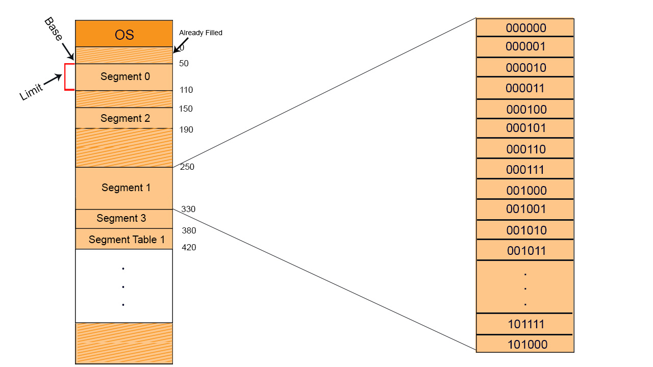
In the diagram given below, we will use the short forms, S is Segment No, d is offset,
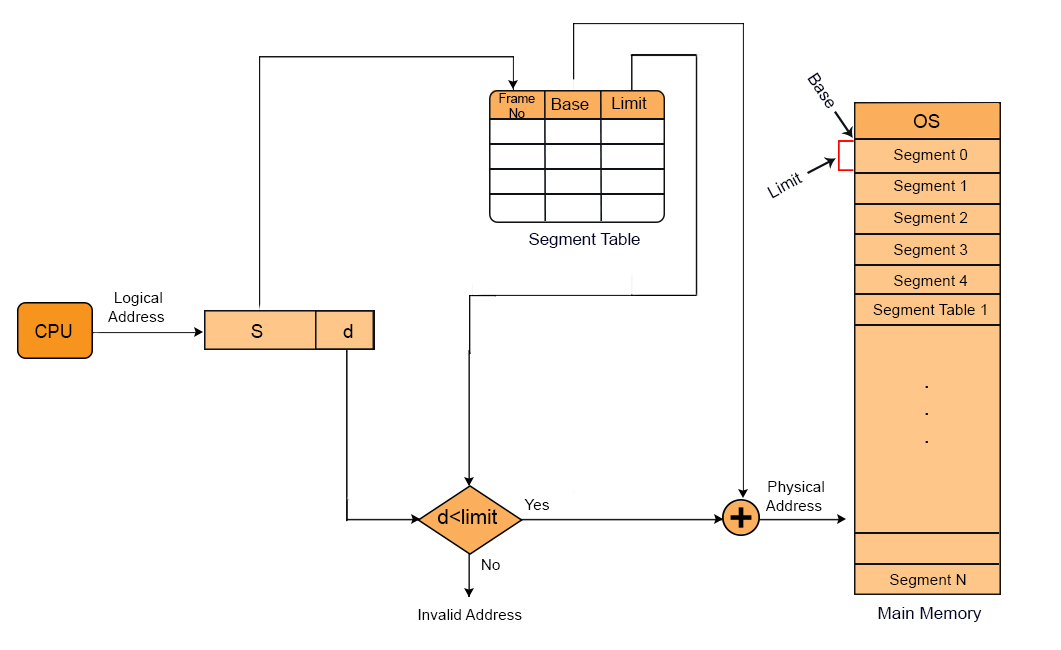
Important: Segments loaded in RAM, may or may not be contiguous.
Suppose a process with its segments loaded in RAM and CPU getting it by generating a logical address as given in the following diagram
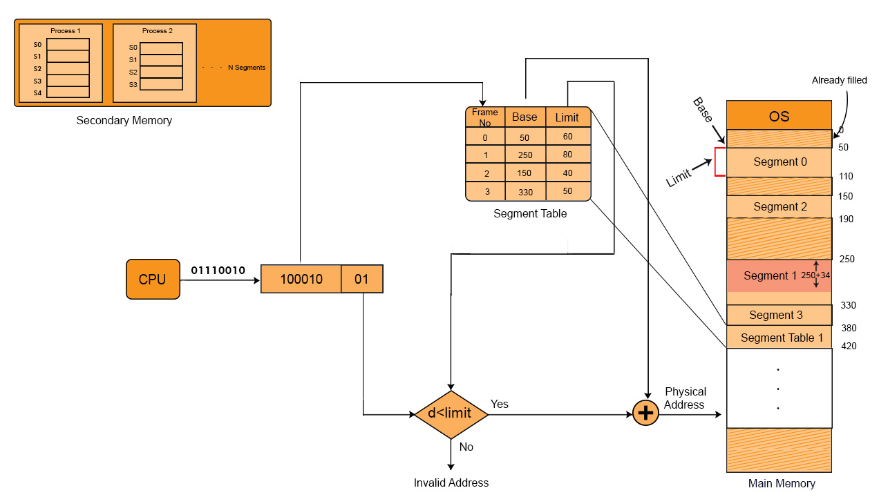
Values of each segment will be like that as shown in the below diagram, in binary representation
Advantages of Segmentation in OS
- Segment table size is less than page table size.
- No internal fragmentation because memory is allocated exactly as per segment size.
- The average size of the Segment is larger than the actual size of the page.
Disadvantages of Segmentation in OS
- It can have external fragmentation.
|
Imagine we have available memory segments of 200 KB, 500 KB, and 300 KB. A process requires a memory segment of 600 KB; however, it cannot be allocated because the free segments are not contiguous. Although the total available memory sums up to 1000 KB, the process cannot utilize it because a single continuous memory segment is necessary. |
- Costly memory management algorithms.
Important Points About Segmentation
Point 01: Program Counter (PC) holds the offset of the current instruction within the segment and generally increments based on the instruction length of a segment, not just a fixed byte increment.
Example:
- If an instruction is 2 bytes long, the PC increases by 2.
- If the next instruction is 4 bytes long, the PC increases by 4.
The CPU keeps fetching and executing instructions until:
- A jump or branch occurs (changing the offset explicitly).
- The segment limit is reached (causing a segmentation fault).
Point 02: Instruction size and offset size depend on the CPU architecture.
- Instruction size varies by CPU: x86 (1–15 bytes), ARM (2/4 bytes), RISC-V (4/2 bytes).
- Offset size depends on CPU mode: 16-bit (2bytes), 32-bit (4bytes), 64-bit (8bytes).
Point 03: Segment limit is checked each time the Program Counter (PC) is incremented to ensure that the CPU does not access memory beyond the segment’s allocated space.
Point 04: CPU generate logical address very time when any instruction of a segement is accessed. Therefore, the total number of logical addresses generated by the CPU would be:
- Total logical addresses = Number of instructions
Point 05: Program counter (PC) Offset, instruction size Relation
- After execution, PC = 1004, pointing to the next instruction.
So, PC is incremented based on instruction size, while offset-size tells the instruction range within a segment.
|